Abstract
The outbreak of the new coronavirus (COVID-19) that emerged in China in December 2019 is the object of strong interest by everybody, and seems to be a very dangerous health problem at the world scale. Journalistic coverage is intense and very anxiety-provoking. The coronavirus outbreak raises many questions (fatality rate, hospital overload,...) that is difficult to answer without a quantitative tool to evaluate the effectiveness of the confinement procedures in particular to control the disease.
For this purpose, a very simple zero-dimensional model of the outbreak has been developped, which can be easily compared to daily observations. From this model, the challenges are clearly highligthed, as well as the chances to block successfully the outbreak prior to the development of a vaccine. The model here presented has been applied successfully to several representative countries where the coronavirus outbreak is well developped: Canada (Quebec), China, France, Germany, Iran, Italy, South-Korea, Spain, Sweden, Switzerland, United-Kingdom and United-State of America. The comparison clearly highlights the effect of a strong quarantine on the long term evolution of the outbreak, long being here about 120 days or 4 months. It is also possible to compare the various fatality rate, and try to understand larges differences between countries concerning the outbreak evolution. Concerning this point, a better undertstanding of the actual outbreak status can be extracted from the analysis of the outbreak in the Diamond Princess boat, where 4000 people where blocked by Japanese authorities during less than a month. Detailed are given in this Sec. 4.2.2 and this led to develop a low fatality rate scenario, applied to France first before to be generalized to other countries after validation.
The approach here presented is valid from the beginning to the end of the outbreak, taking into account of the finite size of the reservoir of people that can be contaminated. It gives therefore an indication if the outbreak will stop (naturally or artificialy thanks to the quarantine) and when, and the total number of people who will die because of the virus. It indicates also time at which the health system will become strongly overloaded. The reservoir effect is accounted by considering the probability of contamination in addition to the rate of contamination.
This note will be regularly updated on the basis on data obtained principally from World Health Organization, Wikipedia®, CDC at Hoston in US. The latter site gives very interesting details to prevent or limit contamination. Another interesting website can be visited here for the outbreak, in particular in Iran. A very well documented worldwide database on the coronavirus outbreak is also available here.
Finally, the code given in Appendix may be used freely (Matlab software required).
Click here to download the pdf version of the report. The HTML version can be easily translated to any languages with Google translator engine inside the web browser. It is available at my personal website.
Note: Date/time in square brackets in the titles of the figures correspond to the date/time at which calculations have been performed.
The contamination process is individual by inter-human contacts. Here the details of the contamination are not considered,. The rate of contamination per people and per day is the main parameter to quantify the growth rate of the contaminated people. It may be adjusted to fit observations, and depending its evolution, it is possible to foresee how the outbreak will evolve, i.e. if it can be controlled or not, manageable or not.
Let suppose that one person is sick but don’t know its own health status. During the incubation period τi, Ni persons will catch the virus by close contact and develop later the disease. The individual mean rate of contamination per person and per day is then
|
| (1) |
knowing the mean incubation time is constant and about τi = 6.4 days from studies of the COVID-19 at Wuhan [7], a number which is subject of very large fluctuations. More references may be found here.
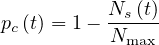
One must introduce also the probability of contamination at time t, pc , related to the chance
that sick people can effectively encounter non-sick people. This parameter plays a minor at the
beginning of the outbreak and is cloe to one. However, it is important to introduce it in order to
simulate the natural end of the outbreak, when all people have been contaminated. Details will be
discussed later. When pc
, related to the chance
that sick people can effectively encounter non-sick people. This parameter plays a minor at the
beginning of the outbreak and is cloe to one. However, it is important to introduce it in order to
simulate the natural end of the outbreak, when all people have been contaminated. Details will be
discussed later. When pc tends towards zero, this mean that herd immunity is close to be
achieved.
tends towards zero, this mean that herd immunity is close to be
achieved.
The daily increase of sick people is then given by the simple law
 | (2) |
and the cumulative number of sick people at time t is
 | (3) |
or
 | (4) |
where Nh is the cumulative number of healed people, and Nd
 is the cumulative number of
deaths. Here, Δt = 1 days. For the COVID-19, Nd ≪ Nh and Nd may be neglected.
is the cumulative number of
deaths. Here, Δt = 1 days. For the COVID-19, Nd ≪ Nh and Nd may be neglected.
The product pc qc
qc ≡ Rc
≡ Rc ∕τi is nothing but the reproductive control number, in presence
of control measures as defined by Kermack & McKendrick. So, according to the above
definitions
∕τi is nothing but the reproductive control number, in presence
of control measures as defined by Kermack & McKendrick. So, according to the above
definitions
 | (5) |
and at the beginning of the outbreak, i.e. Rc = R0 is the well known basic reproduction
number. Since at that time, pc
= R0 is the well known basic reproduction
number. Since at that time, pc = 1,
= 1,
 | (6) |
and if Rc < 1 or Ni <1, the outbreak stops. This corresponds in the model to qc < 1∕τi, or qc < 0.25 approximately with τi = 4 days. So, the longest is the incubation time, the more difficult is the control of the outbreak. This is the reason why the COVID-19 is so difficult to be controlled without a strong confinement of the population. Discussion of R0 is given in Sec. 4.2.1.
In the calculations, it is assumed that the reservoir of people that can be contaminated is initially
almost infinite. Therefore, when the outbreak is starting, pc = 1. If reservoir effects
become significant, like for the passengers in the contaminated cruise liner Diamond-Princess
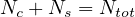
after several days, then the exact balance between people that can be contaminated Nc,
sick people Ns and Nh healed people that cannot be recontaminated (recontamination
seems negligible as far as the virus genetic variability is small) must be properly taken into
account,
= 1. If reservoir effects
become significant, like for the passengers in the contaminated cruise liner Diamond-Princess
after several days, then the exact balance between people that can be contaminated Nc,
sick people Ns and Nh healed people that cannot be recontaminated (recontamination
seems negligible as far as the virus genetic variability is small) must be properly taken into
account,
 | (7) |
with Ntot constant1. This is the classical compartmental approach of the outbreak, in which different populations are considered, which led to the SIR or SEIR models. The reservoir effect can be accounted by the simple relation
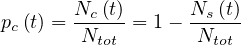 | (8) |
and without any control measures, the outbreak stops if
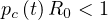 | (9) |
or
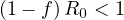 | (10) |
where f = Ns ∕Ntot is the fraction of the population that is naturally immunited (infected or
protected by a vaccine). Therefore,
∕Ntot is the fraction of the population that is naturally immunited (infected or
protected by a vaccine). Therefore,
 | (11) |
Consequently, the larger is R0, the larger the fraction of the immunited population should be to stop naturally the propagation of the virus. So the upper limit of the people that can be contaminated is
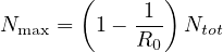 | (12) |
or
 | (13) |
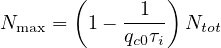
For disease with large R0, a very large fraction of the population should be immunited, almost 95%
for the measles. So, in order in incorporate this limitation, a modified version of pc is considered in
the calculations
is considered in
the calculations
 | (14) |
Finally, if the outbreak is supposed to be suppressed by confinement, the reservoir of non-immunited
people remains very large, and pc ≃ 1.
≃ 1.
The number of healed people is simply described by a delay effect (time to recover)
 | (15) |
where τh is healing time, and δd the fatality rate. While Ns may saturate, Nh
 can
still increase, because of the delay, since Nh
can
still increase, because of the delay, since Nh ≤ Ns
≤ Ns . Usually, as for the flue, τh = 7
days, but here to reproduce the time evolution of the outbreak in China, τh = 14 days
gives better results. This number seems closer to some observations. This means that sick
people recover in 14 days, once symptoms started. This has no impact on the initial rise of
the outbreak. This explain why confinement time τc is about two weeks at minimum,
since
. Usually, as for the flue, τh = 7
days, but here to reproduce the time evolution of the outbreak in China, τh = 14 days
gives better results. This number seems closer to some observations. This means that sick
people recover in 14 days, once symptoms started. This has no impact on the initial rise of
the outbreak. This explain why confinement time τc is about two weeks at minimum,
since
 | (16) |
Finally, the outbreak is ending when the condition
 | (17) |
is fullfiled, i.e. when less than a single person is contaminated.
At t = 0, pc = 1, since nobody is contaminated. At the end of the contamination, since
everybody has been almost contaminated and are supposed to be immunited against the virus,
pc
= 1, since nobody is contaminated. At the end of the contamination, since
everybody has been almost contaminated and are supposed to be immunited against the virus,
pc ≃ 0, which means that the rate of contamination is always naturally decreasing, whatever the
type of outbreak. Since the model here developped has no spatial dimension, only mean values matter,
and one can consider the density of population only. It is therefore assumed that the virus spread
quickly almost uniformly over the whole country, which is a reasonable assumption, since spatially,
the diffusion of the virus follows the Levy flight law : local and slow diffusion by close
contacts described by qc
≃ 0, which means that the rate of contamination is always naturally decreasing, whatever the
type of outbreak. Since the model here developped has no spatial dimension, only mean values matter,
and one can consider the density of population only. It is therefore assumed that the virus spread
quickly almost uniformly over the whole country, which is a reasonable assumption, since spatially,
the diffusion of the virus follows the Levy flight law : local and slow diffusion by close
contacts described by qc combined with very fast long distance diffusion of the disease by
human transportation. It is interesting to observe that the spread of the outbreak of the
coronavirus is identical at the scale of a country (cars, trains,...) or at the scale of the
world (airplane). This the reason why stopping all types of long distance transportation
sytems is the best way to localize the outbreak and hope to have a better control by local
quarantine.
combined with very fast long distance diffusion of the disease by
human transportation. It is interesting to observe that the spread of the outbreak of the
coronavirus is identical at the scale of a country (cars, trains,...) or at the scale of the
world (airplane). This the reason why stopping all types of long distance transportation
sytems is the best way to localize the outbreak and hope to have a better control by local
quarantine.
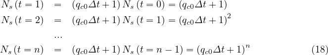
If qc = qc0 is a constant and taking pc = 1, which is the case at the starting point of an
outbreak, prior to first measurements, Eq. 4 corresponds to a geometric series, that can be easily
understood from the elementary process of contamination. Indeed,
= qc0 is a constant and taking pc = 1, which is the case at the starting point of an
outbreak, prior to first measurements, Eq. 4 corresponds to a geometric series, that can be easily
understood from the elementary process of contamination. Indeed,
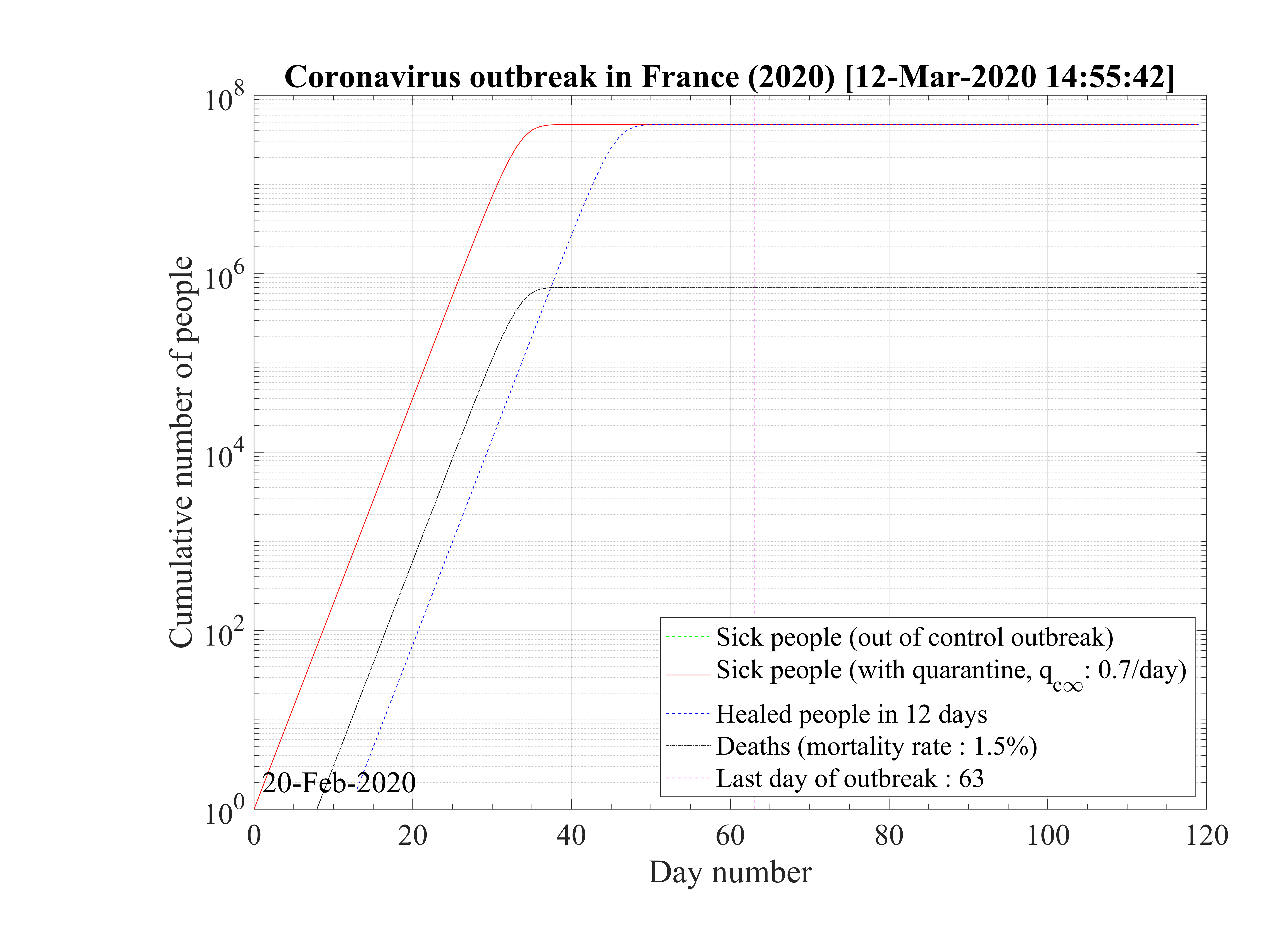
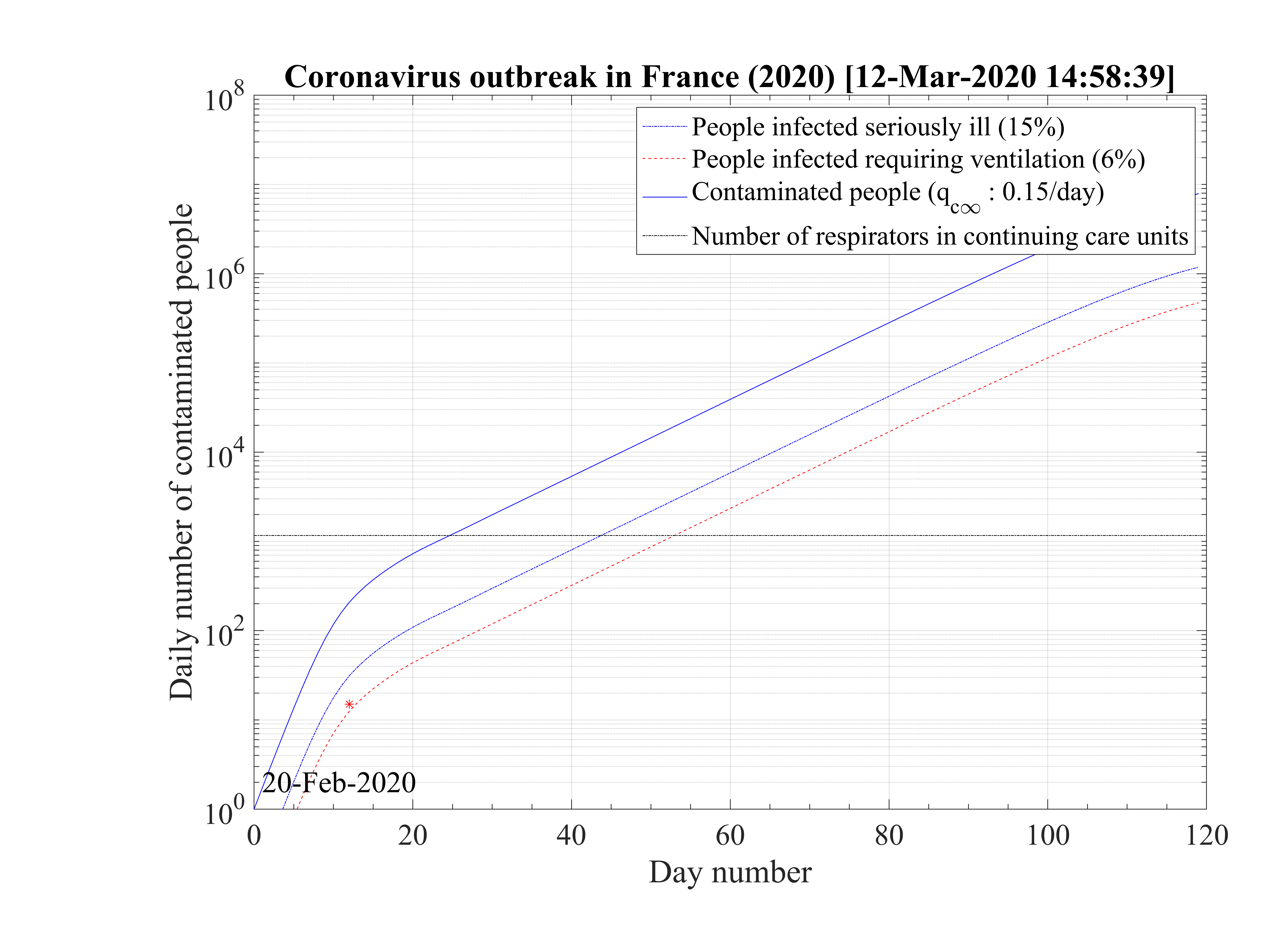
Before entering into the analysis of the results, several values must be given. From Chinese data that can be obtained from the website Johns Hopkins university (USA), the rate of seriously sick people requiring hospitalization is about δvs = 15%, and those requiring in addition an active ventilation is estimated to δvsv = 6% from recent french data, while the mortality rate is about δd = 1.5%, a bit lower than in China. These numbers are just a rough estimate, and may be adjusted for the outbreak in France, in particular for the mortality rate, since advanced medical treatments may be used. It should be recalled that the number of respirators in continuing care units is 1165 in France in January 2020 (offical government number).
From Eq. 4, it is possible to calculate the number of very sick people Nvs requiring
hospitalisation, very sick people requiring intensive care with active ventilation Nvsv
requiring
hospitalisation, very sick people requiring intensive care with active ventilation Nvsv and dead
people Nd
and dead
people Nd . Based on the same approach as for Ns
 , the cumulative number Nvsv
 is
is
 | (19) |
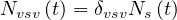
where δvsv is the fraction of sick people that needs ventilation and the daily number of people in the intensive care unit is then
 | (20) |
where Nrvsv is the cumulative number of people that have left the intensive care unit after a time
τvsv, or Nrvsv
is the cumulative number of people that have left the intensive care unit after a time
τvsv, or Nrvsv = Nvsv
Same calculations can be performed with standard care unit, Nvs , while for deaths

 ≃
≃ Nd
Nd if
both . At present time, no specific delay τvs, τvsvand τd is introduced for each sub-population, but
this may be considered, since very sick people requiring intensive care recover or die after 20 days
approximately, three times longer than the standard recovery time τh. Since their fraction is very
small in the early phase of the outbreak dynamics, the feedback may only be expected if the herd
immunity reach its maximum, are if the confinement is successfull to reduce daily variation of Ns. So,
τvs = τvsv = τd = 0 for the early phase of the outbreak. For China, which has almost reached the end
of the outbreak, it is clearly visible that the simulated Nd
if
both . At present time, no specific delay τvs, τvsvand τd is introduced for each sub-population, but
this may be considered, since very sick people requiring intensive care recover or die after 20 days
approximately, three times longer than the standard recovery time τh. Since their fraction is very
small in the early phase of the outbreak dynamics, the feedback may only be expected if the herd
immunity reach its maximum, are if the confinement is successfull to reduce daily variation of Ns. So,
τvs = τvsv = τd = 0 for the early phase of the outbreak. For China, which has almost reached the end
of the outbreak, it is clearly visible that the simulated Nd , which has by definition the same time
dynamics like Ns in the model, is peaked earlier than observed, and then decreases more slowly after
the outbreak peak (see Fig. 38). In the intense phase of the outbreak, it was reported that Chinese
authorities have hidden the actual daily number of deaths, to reduce the political impact of the
outbreak. This option is possible since the daily number of deaths in South-Korea seems to
peak at the same time like Ns, though the low number of deaths makes it difficult to
appreciate, regarding the uncertainty (see Fig. 48). More details will have to be analyse on this
point. Finally, changing τd may have an impact on the value of δd. This may be one of
the difficulty to identify accurately the fatality rate. So far, with τd = 0, the standard
δd values obtained from of more advanced modeling tools allows to reproduce well the
observations.
, which has by definition the same time
dynamics like Ns in the model, is peaked earlier than observed, and then decreases more slowly after
the outbreak peak (see Fig. 38). In the intense phase of the outbreak, it was reported that Chinese
authorities have hidden the actual daily number of deaths, to reduce the political impact of the
outbreak. This option is possible since the daily number of deaths in South-Korea seems to
peak at the same time like Ns, though the low number of deaths makes it difficult to
appreciate, regarding the uncertainty (see Fig. 48). More details will have to be analyse on this
point. Finally, changing τd may have an impact on the value of δd. This may be one of
the difficulty to identify accurately the fatality rate. So far, with τd = 0, the standard
δd values obtained from of more advanced modeling tools allows to reproduce well the
observations.
Due to possible onset of efficient medications during the outbreak, δvs, δvsv and δd may themselves
be time dependent. Such a possibility is not yet considered but may be easily introduced in the
calculations. Regarding the uncertainty from daily variations of Ns , this may be considered at the
end of the outbreak only. None of the outbreak simulations are able to be accurate thanks to this
problem, at the early stage.
, this may be considered at the
end of the outbreak only. None of the outbreak simulations are able to be accurate thanks to this
problem, at the early stage.
Finally, the quarantine policy, i.e. the social interaction is modeled by a simple smooth step or sigmoid function of the form
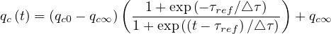 | (22) |
in order to mimic the usual observed decrease of qc . Significance of parameters are simple: qc0 and
qc∞ are respectively the initial and final rates of contamination, τref is the mean time at which the
slope is maximum between the two levels of the contamination rates, and △τ describes the time
evolution at which qc
. Significance of parameters are simple: qc0 and
qc∞ are respectively the initial and final rates of contamination, τref is the mean time at which the
slope is maximum between the two levels of the contamination rates, and △τ describes the time
evolution at which qc evolves from qc0 to qc∞. It is important to recall that R0 = qc0τi, and
Rc = qcτi.
evolves from qc0 to qc∞. It is important to recall that R0 = qc0τi, and
Rc = qcτi.
At t = 0, qc = qc0, while limt→∞qc
 = qc∞. If the quarantine is realeased at a time trel, and
the outbreak restarts, the above model may still be applied, but with values corresponding to the new
situation. The corresponding formula is then
= qc∞. If the quarantine is realeased at a time trel, and
the outbreak restarts, the above model may still be applied, but with values corresponding to the new
situation. The corresponding formula is then
 | (23) |
for t > trel. It is interesting to observed that once the outbreak starts, qc0 ≃ 0.75 - 1 in almost all countries. If the population has not realized that an outbreak is developing, it stays at the initial value during a long period. Then the population starts to self-protect, and qc∞≃ 0.2 - 0.3. The time τref is a good indicator at which this occurs, and △τ the speed at which the information propagates in the population. Roughly, △τ ≃ 2 (See Table 1). After, this natural qc∞ stays almost constant, and from its value, one can derive if there is a chance that the outbreak will slow-down or not, i.e. if it will end naturally by herd immunity or by actively stopping the individual contamination, i.e. reducing social interactions. This is the purpose of this model.
In the case of change of qc at a given time t = trel, the continuity of qc
 leads to the
relation
leads to the
relation
 | (24) |
so it is easy to determine any time t = trel a change in the outbreak evolution.
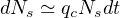
When △t → 0, Eq. 2takes the differential form
 | (25) |
Let’s consider first the simple case where Nd ≪ Nh ≪ Ns, and pc = 1,which is the case in the early phase of outbreak or with a strong confinement, such that Ns + Nh + Nd ≪ Ntot. In this case;
 | (26) |
or
 | (27) |
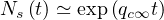
Introducing the smooth step function Eq. 22,
![[ ( ) ]
dNs- --1+-exp-(--τref∕△-τ)-
Ns = (qc0 - qc∞ ) 1 + exp((t - τref)∕△τ) + qc∞ dt](coronavirus68x.png) | (28) |
or
 | (29) |
and integrating both sides
 | (30) |
gives
 | (31) |
since Ns = 1.
= 1.
The indefinite integral being
 | (32) |
the integrated number of contaminated people is then
![( ( )) [ ( ( )) ( ( ))]
ln Ns = (qc0 - qc∞) 1+ exp - τref t- △ τ ln 1 + exp t-- τref + △ τ ln 1 + exp - τref +qc∞t
△τ △ τ △τ](coronavirus74x.png) | (33) |
so at t = 0
![( ( ) ) [ ( ( )) ( ( ) )]
ln Ns(t = 0)) = (qc0 - qc∞ ) 1 + exp - τref - △ τ ln 1 + exp - τref + △τ ln 1+ exp --τref = 0
△ τ △τ △ τ](coronavirus75x.png) | (34) |
and Ns = 1 is well recovered.
Therefore
![[ ( ( )) [ ( ( )) ( ( ) )] ]
N (t) = exp (q - q ) 1 + exp - τref- t- △τ ln 1+ exp t--τref + △ τ ln 1 + exp --τref + q t
s c0 c∞ △ τ △ τ △ τ c∞](coronavirus77x.png) | (35) |
or
![[ ( ( τref )) [ ( (t- τref)) ( (- τref) )] ]
Ns(t) = exp (qc0 - qc∞ ) 1 + exp - △-τ t- △τ ln 1+ exp --△-τ-- + △ τ ln 1 + exp -△-τ- + qc∞t](coronavirus78x.png) | (36) |
which means without people recovering, Ns is indefinitely growing if qc∞ > 0.
If t ≪ τref,
![[ ( ( τ )) [ ( ( τ ) ) ( ( - τ )) ] ]
Ns(t) ≃ exp (qc0 - qc∞ ) 1 + exp --ref t- △τ ln 1+ exp - -ref- + △ τ ln 1+ exp --ref + qc∞t
△ τ △ τ △ τ](coronavirus80x.png) | (37) |
or
![[ ( ( ) ) ]
Ns(t) ≃ exp (qc0 - qc∞ ) 1 + exp - τref t+ qc∞t
△ τ](coronavirus81x.png) | (38) |
or
![[( ( ( )) ) ]
τref
Ns (t) ≃ exp qc0 + (qc0 - qc∞) 1+ exp - △τ t](coronavirus82x.png) | (39) |
and if qc∞≪ qc0,
Ns ≃ exp ≃ exp![[ ( ( )) ]
qc0 2+ exp - τref t
△τ](coronavirus84x.png)
|
Conversely, if t ≫ τref, Eq. 36 simplifies to
![[ ( ( τref)) [ ( ( - τref) )] ]
Ns (t) ≃ exp (qc0 - qc∞) 1+ exp --△τ- τref + △τ ln 1+ exp -△-τ- + qc∞t](coronavirus85x.png) | (40) |
and even if qc0 ≫ qc∞, at a given time t,
 | (41) |
So the importance of the residual contamination rate qc∞ on the long term evolution. As expected for
qc∞ = 0, Ns becomes constant.
The peak of the outbreak is the key time at which the daily number of contaminated people starts to decrease. It can be the consequence of an herd immunity but also enforced by a strict confinement of people to reduce interactions, namely qc. This case is not considered here.
Since the delay of recovery τh is long enough for Nd ≪ Nh ≪ Ns, the time at which the peak can be estimated with the approximation Nh = Nd ≃ 0. After the peak, the dynamics of the outbreak fully must consider Nh and Nd in the calculations and the equation to be solved is
 | (42) |
Thanks to the above approximation that is specific to the coronavirus outbreak, τpeak is
determined by the equation Ns′′ = 0. From Eq. 36,
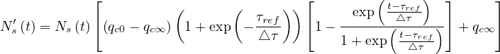 | (43) |
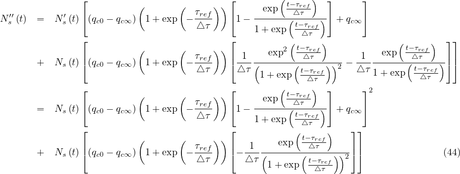
If qc∞ < qc0, there exists always a peak of the outbreak. Time to reach the peak from the onset of the quarantine is therefore
![[ 1 q ]
τpeak - τref ≃ △ τ ln---c20-
△τ qc∞](coronavirus95x.png) | (48) |
in the limit τref ≫△τ and qc∞≪ qc0. Since for most countries, qc0 ≃ 1 and qc∞≃ 0.01 to control
the outbreak rapidly is to lower △τ. So, to set-up a strong quarantine on the shortest possible time
scale. For △τ = 1, τpeak - τref ≃ ln![[ +4]
10](coronavirus96x.png) ≃ 9 days. In general, τpeak - τrefis about two
weeks. It worth to note that τpeak is very sensitive to simulation parameters, and the if
assumptions are not satisfied, the exact solution must be used instead of the approximate
one.
≃ 9 days. In general, τpeak - τrefis about two
weeks. It worth to note that τpeak is very sensitive to simulation parameters, and the if
assumptions are not satisfied, the exact solution must be used instead of the approximate
one.
At time corresponding to the outbreak peak, the outbreak speed is the faster, i.e.
dNs∕dt = qc is maximum. As far as Ns′′′
 > 0, it means that the outbreak is increasing,
while the point at which Ns′′′
> 0, it means that the outbreak is increasing,
while the point at which Ns′′′ = 0 indicates that it starts to slow-down.
The contamination rate qc∞ is the key parameter to decide if it is possible to control the outbreak, namely stop it, regarding the initial value qc0 which gives the force of the outbreak. Such an approach require to solve Eq. 45, and depending the ratio qc∞∕qc0, to find if a solution τpeak. Regarding the sensitivity of the Eq. 45, only a numerical determination can be carried out, as it has been done for France in Sec. 3.1.3
Far from the outbreak peak, as reached by China and South-Korea, the daily number of cases or deaths is not going to zero as expected, but remains at a residual level, about 100 cases per day for both countries (30th of March). Such a persistence observed during more than 10 days indicates the high risk that the outbreak can restart. If △Ns is constant and independent of time, in the limit where pc ≃ 1 and qc = qc∞ it means that
 | (49) |
or in a differential formulation
 | (50) |
which gives
 | (51) |
so Nsshould increase linearly with time, and since Nh = Ns
= Ns ,
,
 | (52) |
so
 | (53) |
If qc∞ < 1∕τh, Ns - Nh
- Nh < 1, so Ns
 - Nh
- Nh are almost identical, as expected, and the
differene is constant. All quantities are linearly growing, Ns
are almost identical, as expected, and the
differene is constant. All quantities are linearly growing, Ns , Nh
, Nh , but also the cumulative
number of deaths.
, but also the cumulative
number of deaths.
The application of the epidemic model has been applied to the seven main countries concerned by the coronavirus outbreak, i.e. China, France, Iran, Italy, South-Korea, Switzerland, and United-State of America. More recently, two other countries have been added: Germany and United-Kingdom, and the Quebec province of Canada.
China was the first country concerned by the outbreak which started at Wuhan, in December 2019. During a quite long period, the disease was underground, and exceptionaly strong quarantine was applied by end of January 2020. In Italy, the same kind of underground evolution of the disease is observed during almost two weeks, before a sudden strong growth of the number of confirmed cases, in almost one day.
This day is considered in the calculations as the reference day. Such an evolution is also observed in France, USA, Germany, United-Kingdom and especially in South-Korea where it indicates how easily can the outbreak restart after a full control. The robustness of the outbreak is therefore in question. Likely, this early phase corresponds to inported cases, from people travelling by airplane that can be easily isolated. The effective start of the outbreak is an indication that the disease becomes domestic, and conditions for a local control are becoming much more difficult.
The equations have been translated into a Matlab script available in Appendix to analyse the impact
of various parameters. Data are obtained from news website reporting official government
press conferences. The initial number of contaminated people is taken Ns = 1, but
day 0 is unknown. It is adjusted to have the best fit of initial observed values of Ns
= 1, but
day 0 is unknown. It is adjusted to have the best fit of initial observed values of Ns .
This uncertainty has a wek impact on the overall conclusions. Just absolute numbers may
change slightly. From the growth rate of Ns at the early stage of outbreak, qc0 ≃ 0.70.
This means that one sick person can contaminate 4.5 persons in the incubation time so a
bit less than one person per day. The french population is taken to Ntot = 6.7 × 10+6
inhabitants.
.
This uncertainty has a wek impact on the overall conclusions. Just absolute numbers may
change slightly. From the growth rate of Ns at the early stage of outbreak, qc0 ≃ 0.70.
This means that one sick person can contaminate 4.5 persons in the incubation time so a
bit less than one person per day. The french population is taken to Ntot = 6.7 × 10+6
inhabitants.
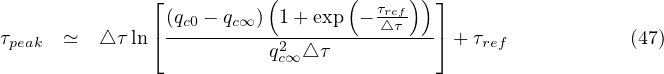
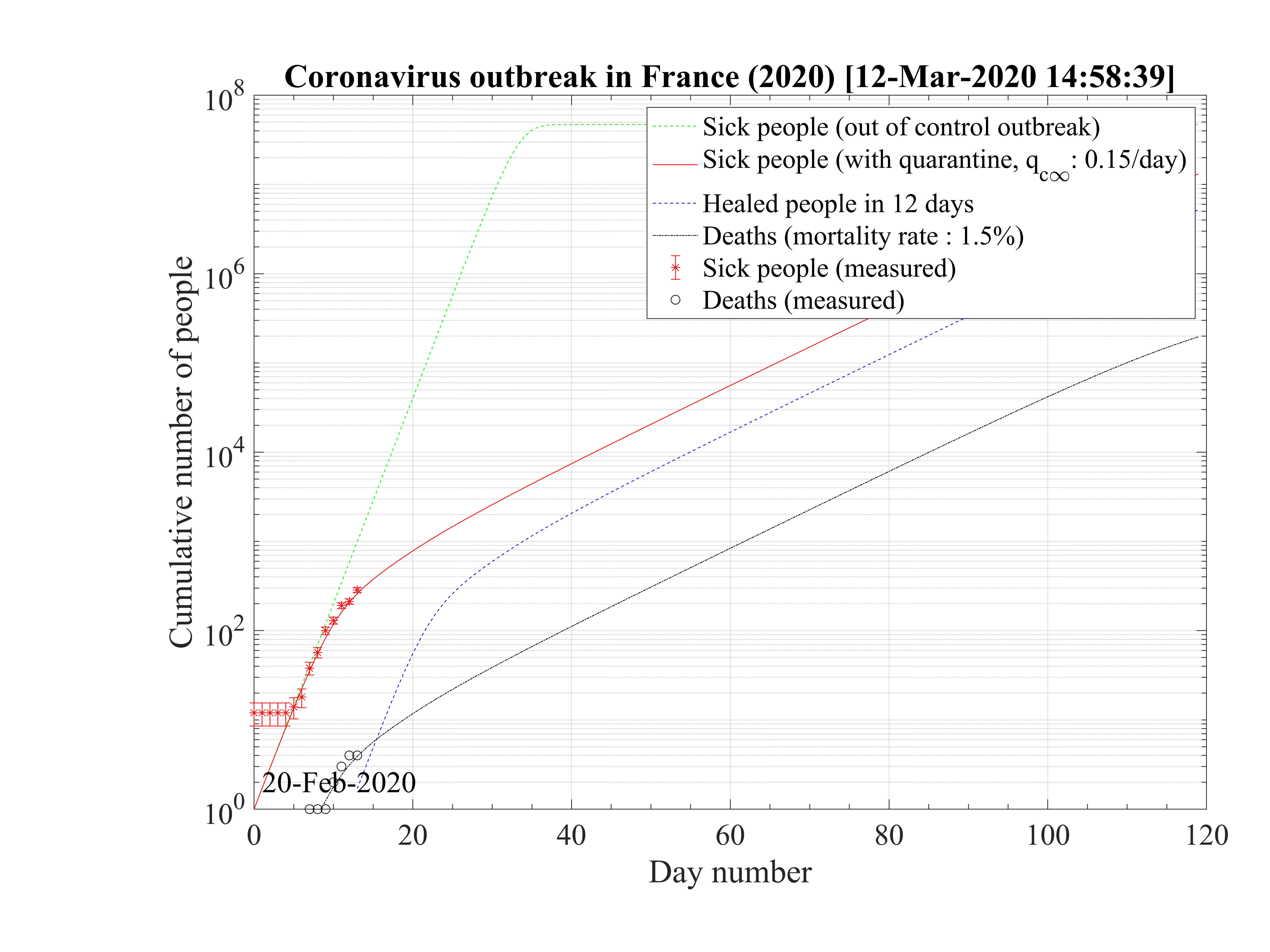
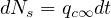
Considering that nothing is done against the outbreak and qc = qc0 = 0.70, the natural last day
of the outbreak is 63, all people have been contaminated, and the number of people who died is one
million approximately as shown in Fig. 1. The evolution of qc
= qc0 = 0.70, the natural last day
of the outbreak is 63, all people have been contaminated, and the number of people who died is one
million approximately as shown in Fig. 1. The evolution of qc is indicated in Fig. 2. The number of
very sick people requiring continuous artificial ventilation is exceeding the total number of available
respirators in continuing care units 18 days after the beginning of the outbreak, with a maximum of
nvsvmax = 2.7 × 10⁶, which is dramatically high as compared to operational limits (Fig. 3). Most
of the people won’t have any respirator, and the risk of death will be likely enhanced.
is indicated in Fig. 2. The number of
very sick people requiring continuous artificial ventilation is exceeding the total number of available
respirators in continuing care units 18 days after the beginning of the outbreak, with a maximum of
nvsvmax = 2.7 × 10⁶, which is dramatically high as compared to operational limits (Fig. 3). Most
of the people won’t have any respirator, and the risk of death will be likely enhanced.
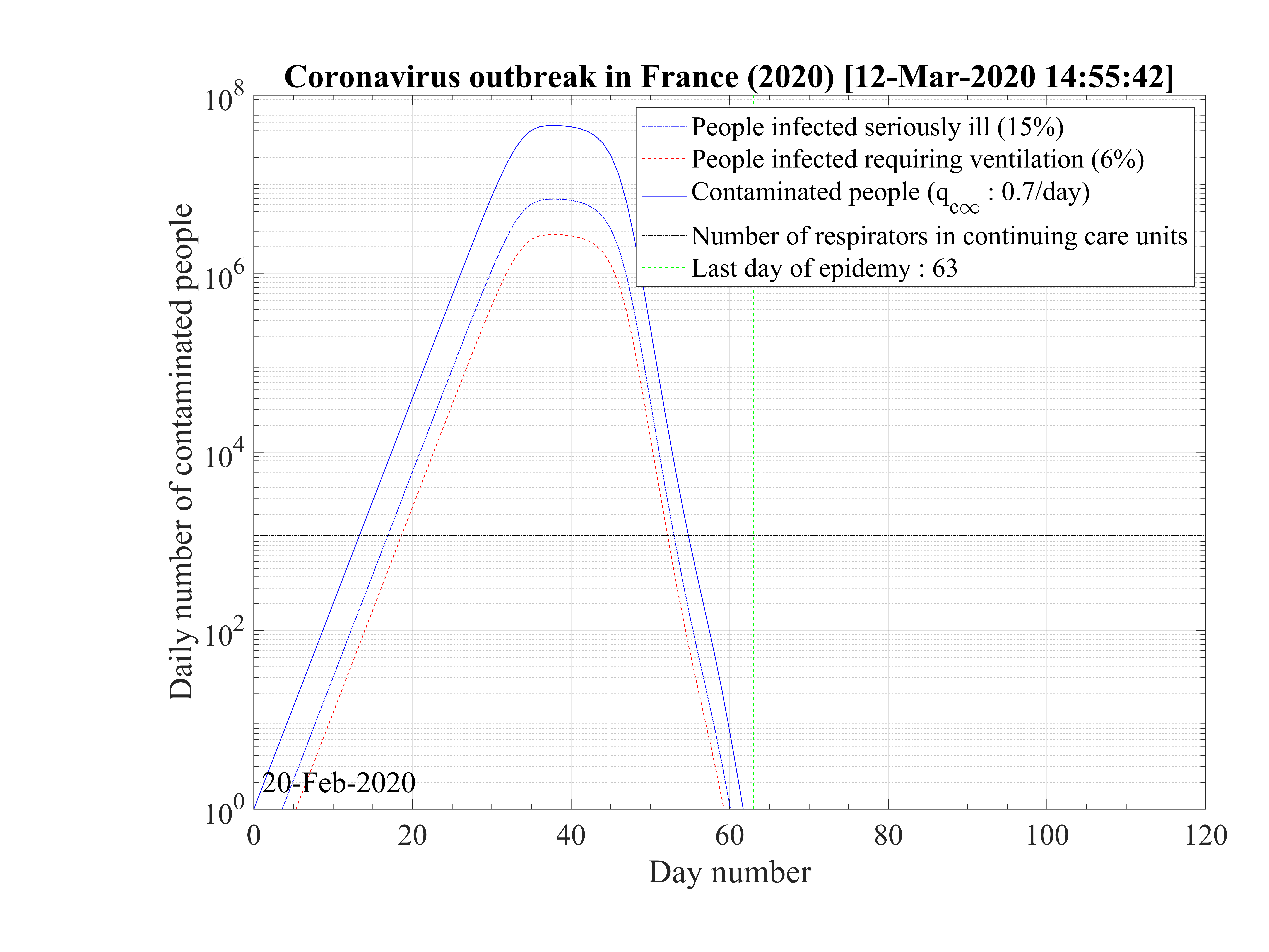
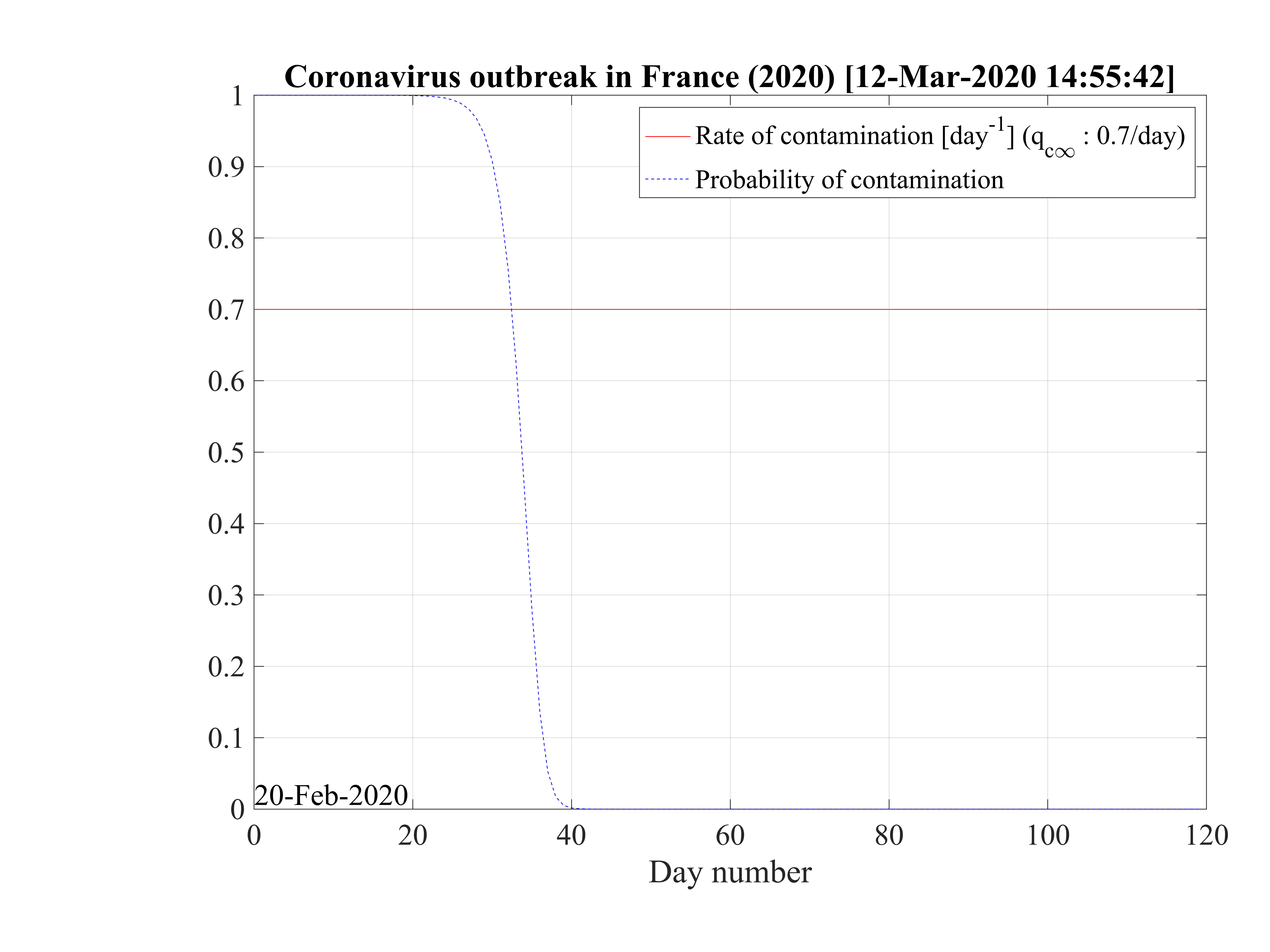
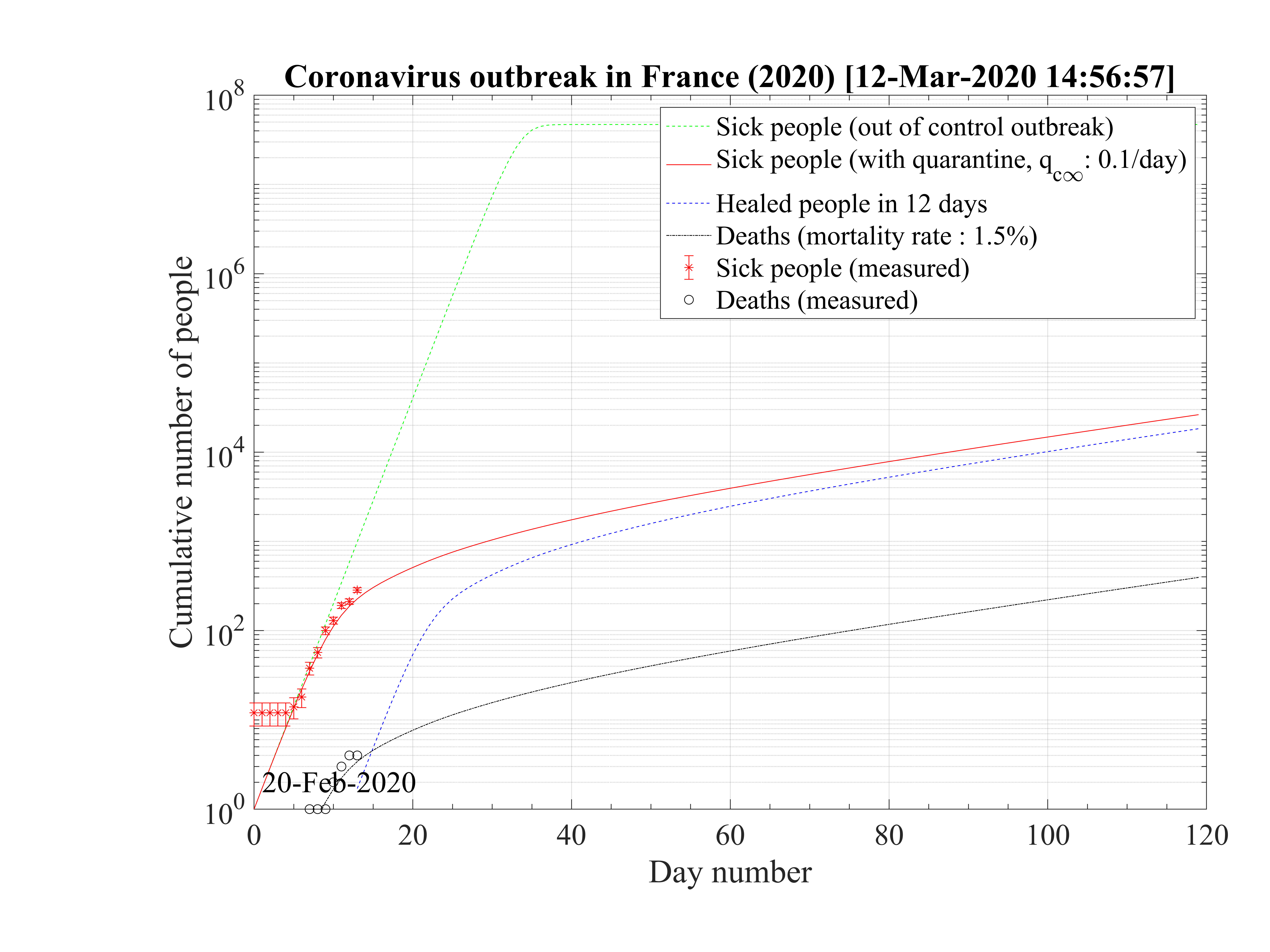
Regarding the outbreak status the 4th of March 2020, qc∞ falls down to 0.1 approximately, as shown in Fig. 5, and the outbreak seems under reasonable control as shown in Figs. 4. The last day of the outbreak is 87, and the maximum number of persons that are sick is about 311 (Fig. 6). The number of people requiring ventilation remains always well below the capacity of continuing care units. This case may be easily managed by the country.
This results principaly from the setup of a quarantine procedure, by tracking sick people and also
people that may have been is close contact to the well identified sick people. Therefore qc is quickly
decreasing. This is a critical step for an efficient quarantine, and the possibility to slow down the
outbreak. In addition, non contaminated people must reduce themselves the risk of contimation
(washing hands periodically, one meter distance minimum, no hand shaking and no kiss, ...), while
isolated ones must accept to be in quarantine, for the general interest of the society, especially in
countries where individual freedom matters. This acceptance is crucial in the success of the
method.
is quickly
decreasing. This is a critical step for an efficient quarantine, and the possibility to slow down the
outbreak. In addition, non contaminated people must reduce themselves the risk of contimation
(washing hands periodically, one meter distance minimum, no hand shaking and no kiss, ...), while
isolated ones must accept to be in quarantine, for the general interest of the society, especially in
countries where individual freedom matters. This acceptance is crucial in the success of the
method.
The result is a fast drop of qc leads to the clear inflexion of the cumulative number of sick
people, as shown in Fig. 4. The 4th of March, the reduction of the number of contaminations is about
1000 persons, as compared to the case of an uncontrolled outbreak. The number of dead people is also
well reproduced by the model.
leads to the clear inflexion of the cumulative number of sick
people, as shown in Fig. 4. The 4th of March, the reduction of the number of contaminations is about
1000 persons, as compared to the case of an uncontrolled outbreak. The number of dead people is also
well reproduced by the model.
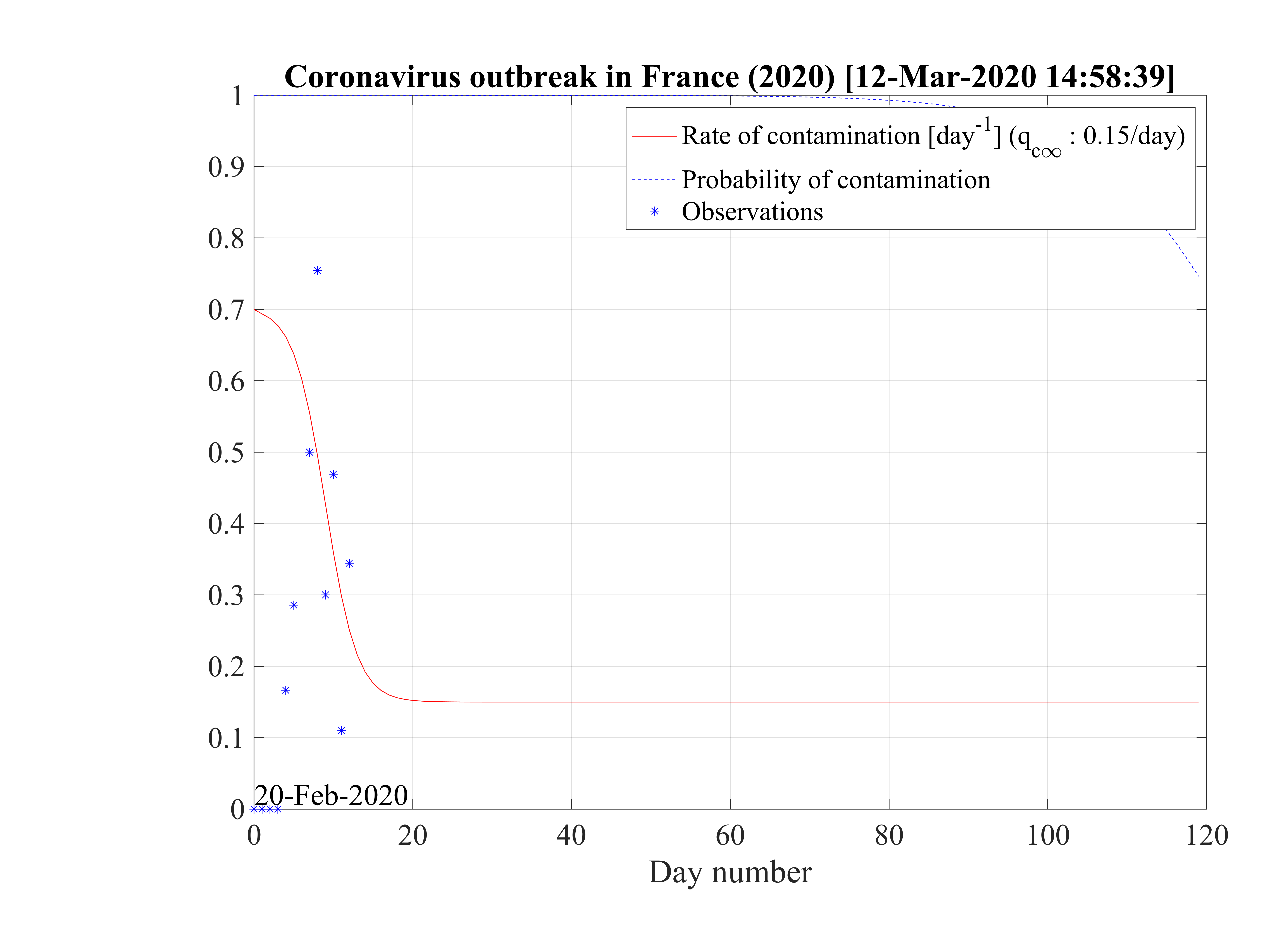
In the simulation, the drop of qc has been modeled from Eq. 22, with τref = 10 days, the
sharpness in time of the decrease is reproduced by △τ = 2 days, and the residual value of the
contamination rate per day and per person is qc∞. This is an arbitrary number which has a crucial
importance on the long term evolution of the outbreak. As shown in Fig. 4, the quarantine leads to a
saturation of the number of sick people.
has been modeled from Eq. 22, with τref = 10 days, the
sharpness in time of the decrease is reproduced by △τ = 2 days, and the residual value of the
contamination rate per day and per person is qc∞. This is an arbitrary number which has a crucial
importance on the long term evolution of the outbreak. As shown in Fig. 4, the quarantine leads to a
saturation of the number of sick people.
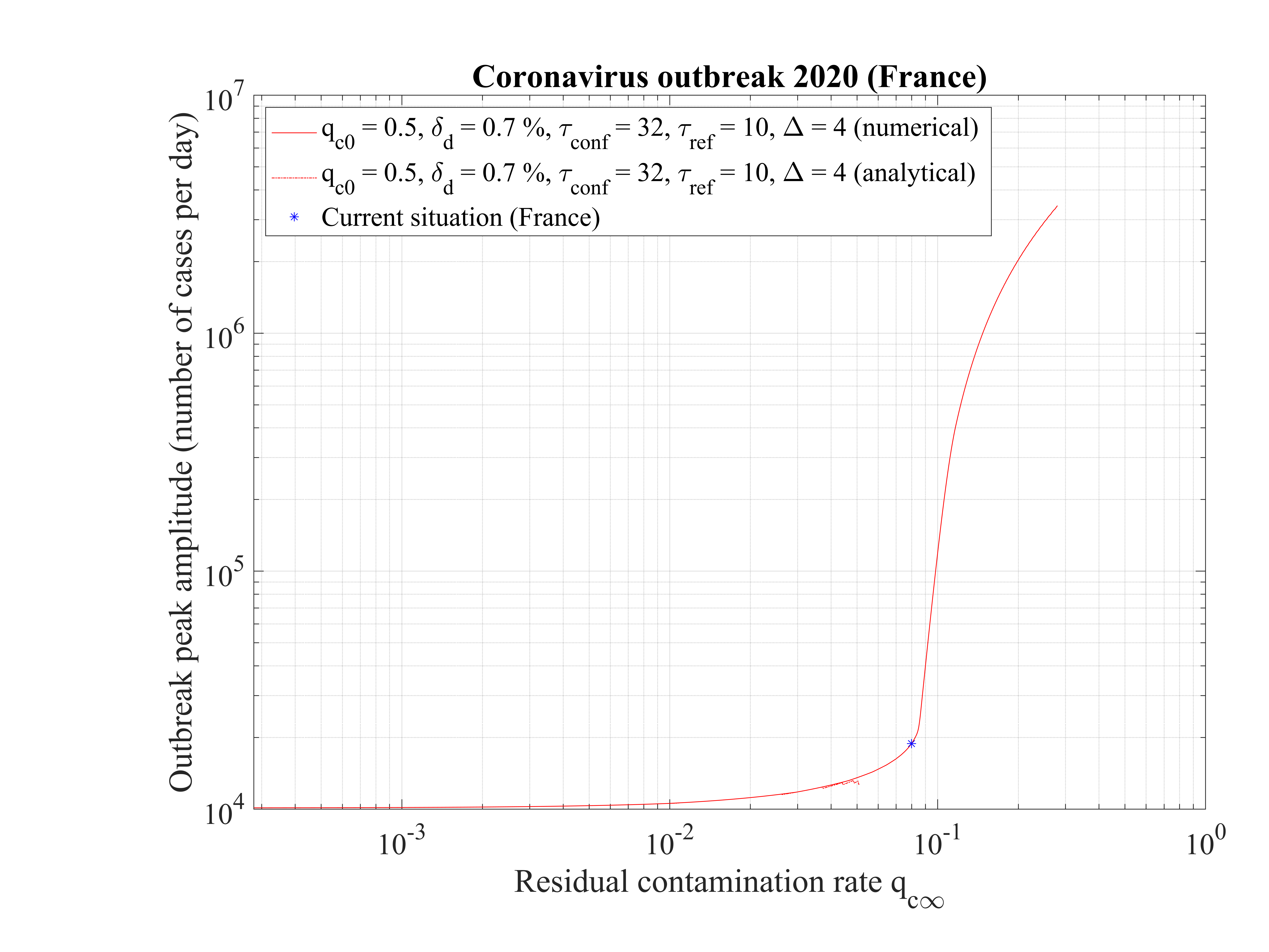
The sensitivity of the model to qc∞ is a critical issue for the control of the outbreak. If it is raised to qc∞ = 0.15 as shown in Fig. 8, which is still compatible with observations at the 4th of March 2020, as seen in Fig. 7, the number of contaminated people is increasing up to reach Ntot, which means that all the country will be contaminated, but on a much longer time scale as compared to the case without a quarantine. The outbreak is not under control but remains manageable, as shown in Fig. 9, since the growth rate of people that are requiring a respirator is small. Their are some margins to increase the number of respirators in continuing care units. This should be the realistic approach at present time.
Each additional day after the 4th of March give precious details on the effective control of the outbreak, and issues in the coming weeks. Data can be added easily in the script to follow the evolution and understand the outbreak. In particular, the function given by Eq. 22 may have to be changed after a given time if necessary.
The 6th of March, the growth of contaminated people is very important, and is qc∞ = 0.25 must be chosen to reproduce observations with the model, a much higher value than initialy estimated the 4th of March. This highlight the impossibility to extrapolate with strong confidence what will be the evolution of the outbreak. Here the model helps just to extrapolate if nothing is done at a given day.
Thanks to the observations, the outbreak is therefore not under control, and will become not manageable 28 days after the beginning of the outbreak, so at the end of March, if nothing is done. The number of sick people will exceed ten thousands after 30 days, so at about the 20th of March. Almost everybody will be concerned and be contaminated in hundred days, and at that time, the number of deaths will reach about 714000. This number should be compared to the number of deaths because of the flue in 2019, which is 8100. So hundred times more..., which illustrates the severity of the outbreak. The end of the outbreak will last in a year approximately.


From the high fatality rate scenario, it is possible to evaluate the effect of the reduction of qc∞ from
qc0 down to 0 on the duration of the outbreak, the day at which the outbreak peaks and the total
number of deaths. Initial simulation parameters that are not changing in the scan, are :
qc0 = 0.7, qc∞ = 0.27, τref = 10 days, △τ = 2 days. Since the amplitude of the outbreak peak
depends of the reference day, calculation are performed with a second set of paremeters
starting at day 24 (16th of March) at which confinement is decided in France. Initial ones are
unchanged, while in the phase, i.e. after day 24, qc0 is deduced from continuity of qc ,
τref = 10 days and △τ = 10 days, the latter being longer to reflect the longer decay of the
outbreak.
,
τref = 10 days and △τ = 10 days, the latter being longer to reflect the longer decay of the
outbreak.
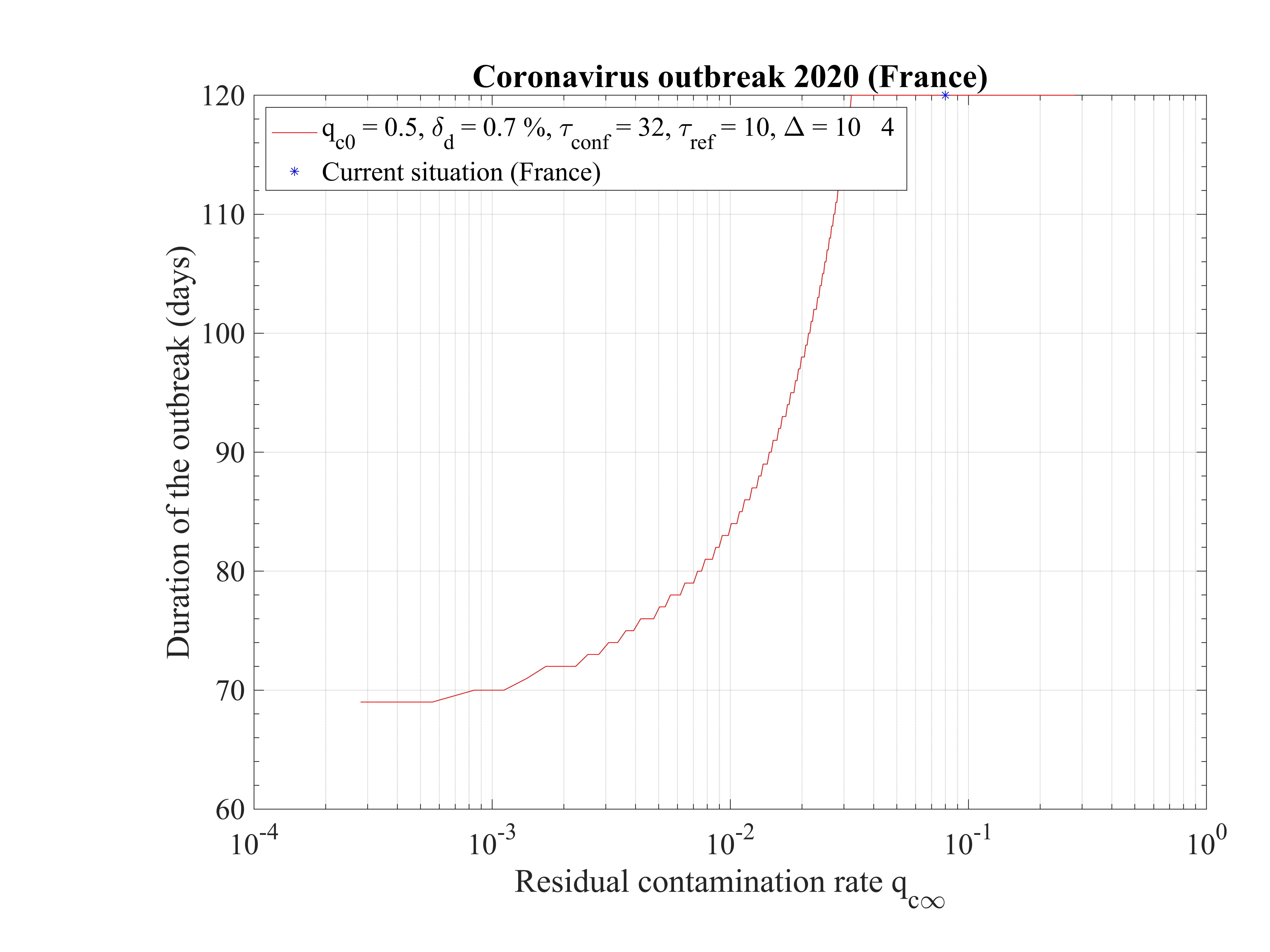
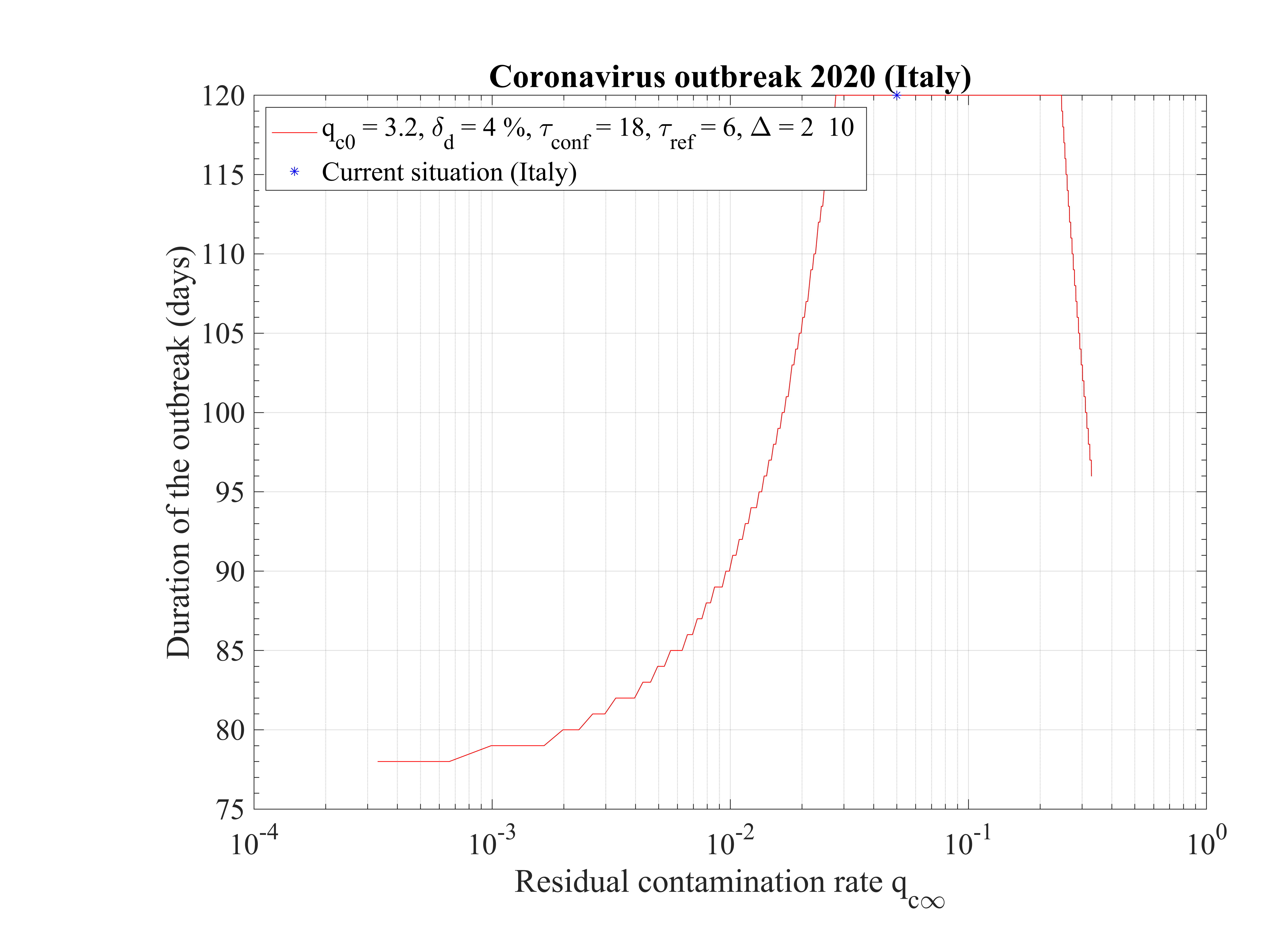
As shown in Fig. 15, the duration of the outbreak starts to increase when qc∞ is decreased and exceeds rapidly the the upper limit of 120 days of the study here considered. As far as qc∞ > 0.05, the outbreak is not controlled by confinement but naturally controlled by herd immunity. If in the confinement phase qc∞ is divided by more than a factor 5, the outbreak can be controlled, the smaller is qc∞ the shorter is the outbreak. For qc∞ = 0.05, the outbreak lasts more than 120 days from the time at which it started (simulation limit).
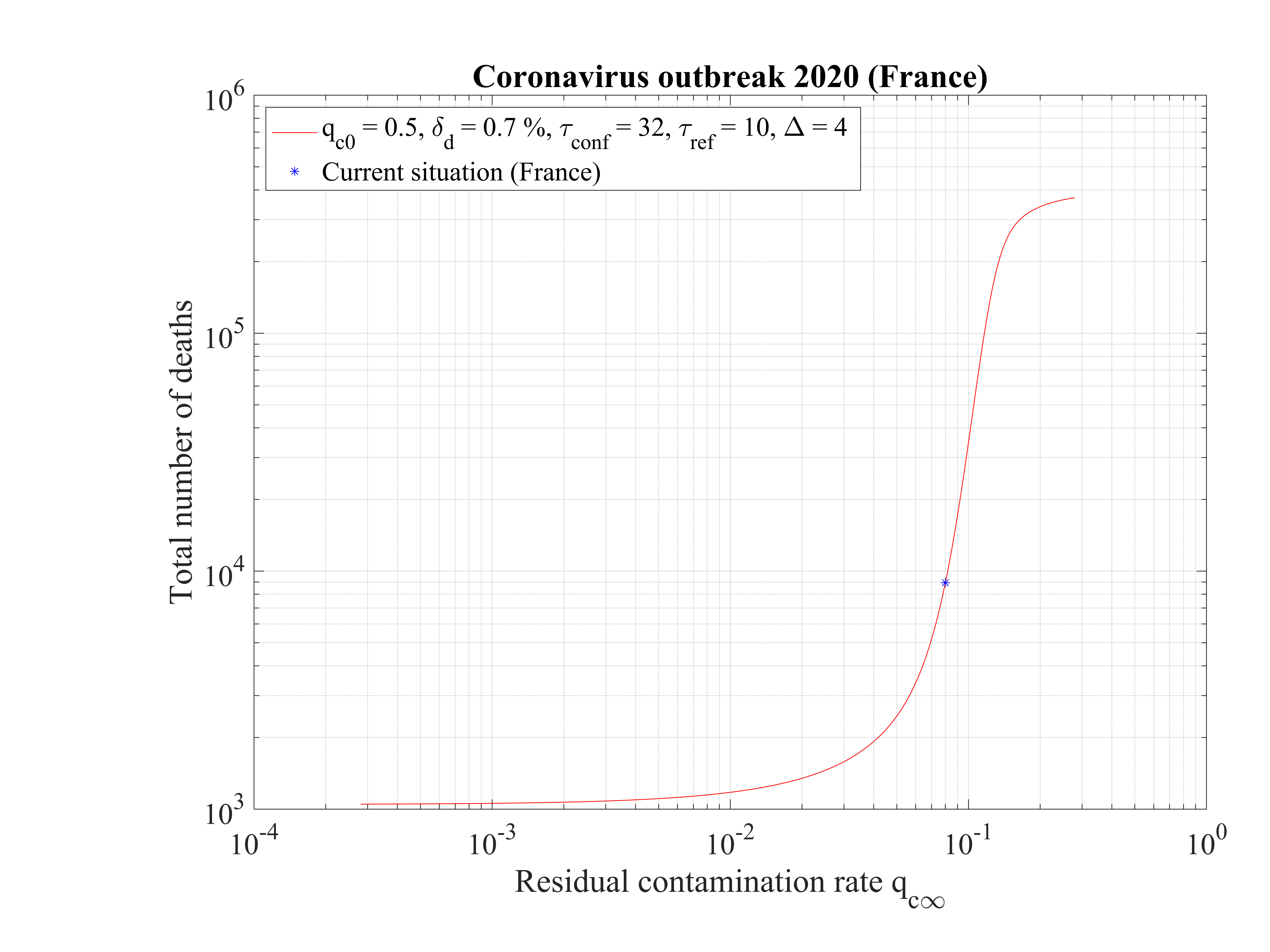
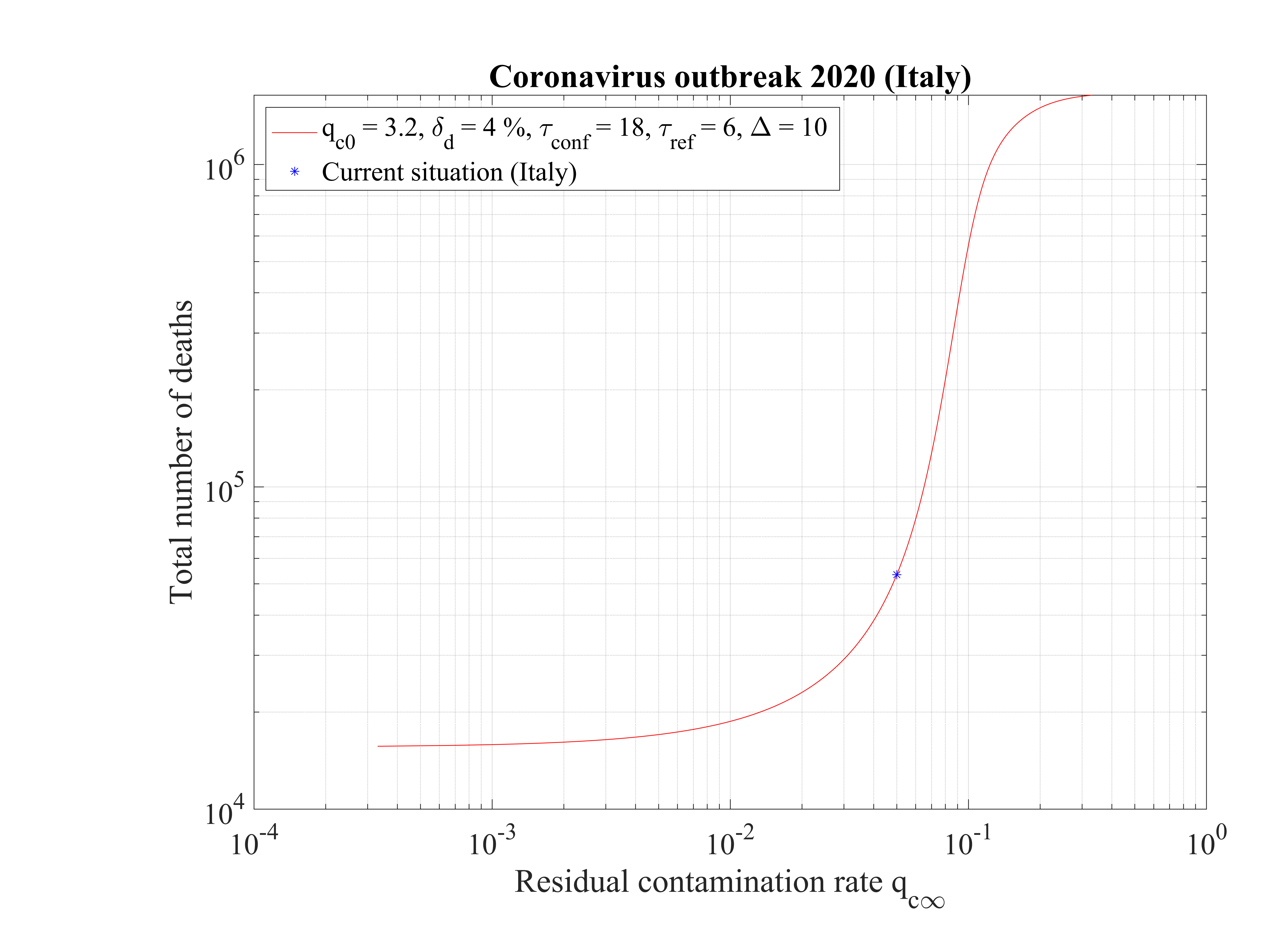
In Fig. 16, the total number of deaths is shown. For qc∞ = 0.05, it is down to 15000 approximately. It rises quickly if the outbreak is not controlled, i.e. qc∞ > 0.05.
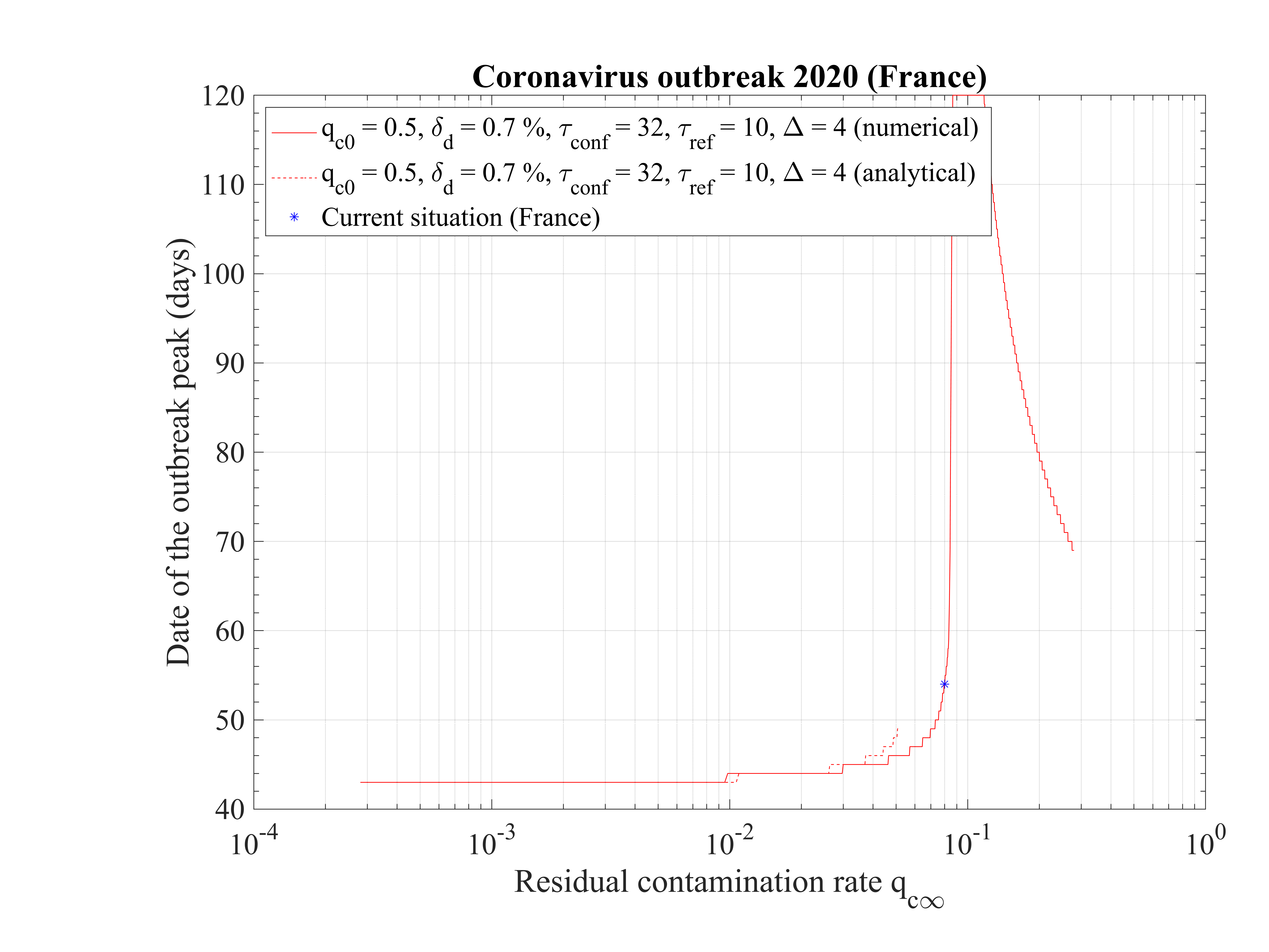
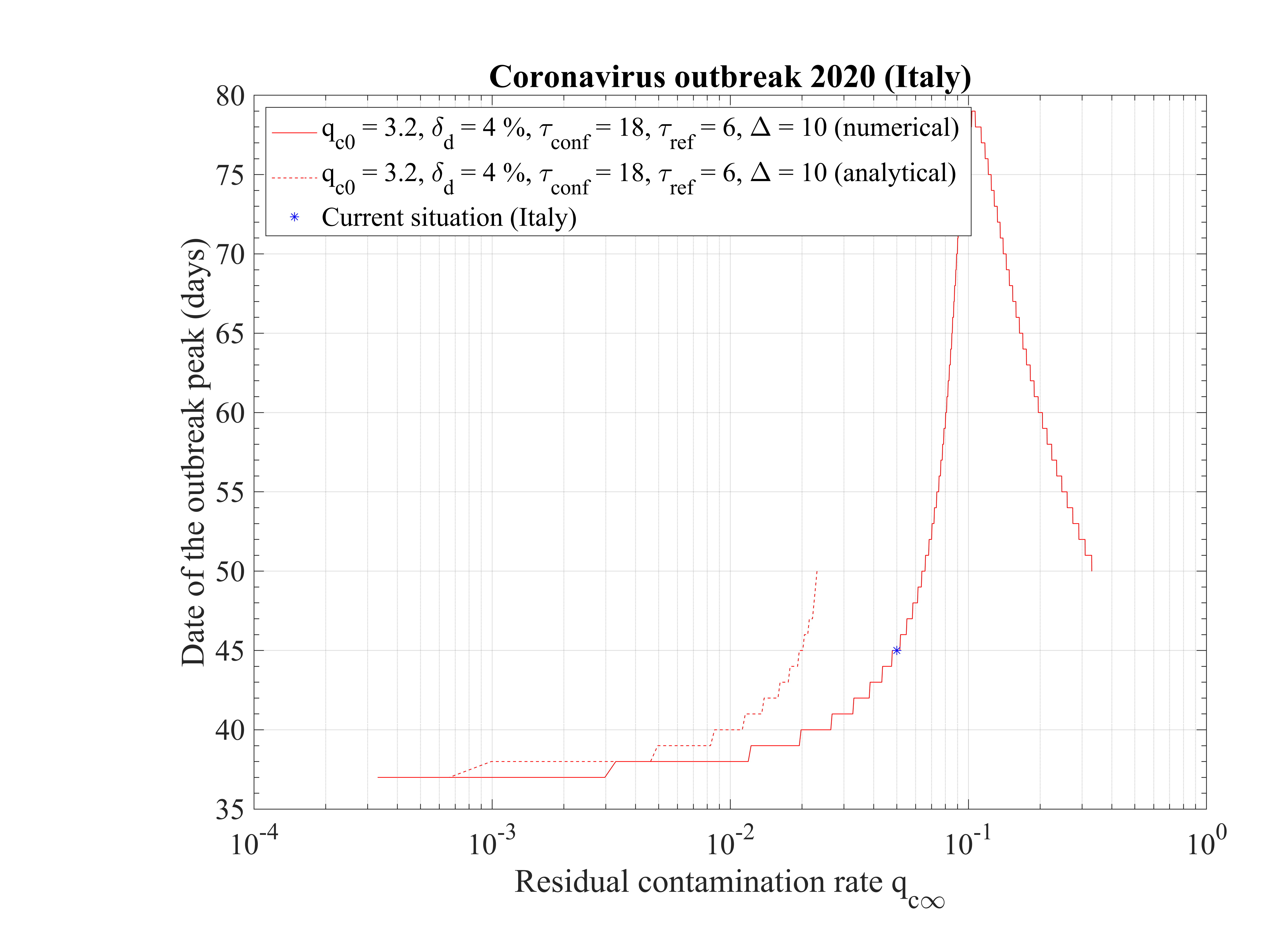
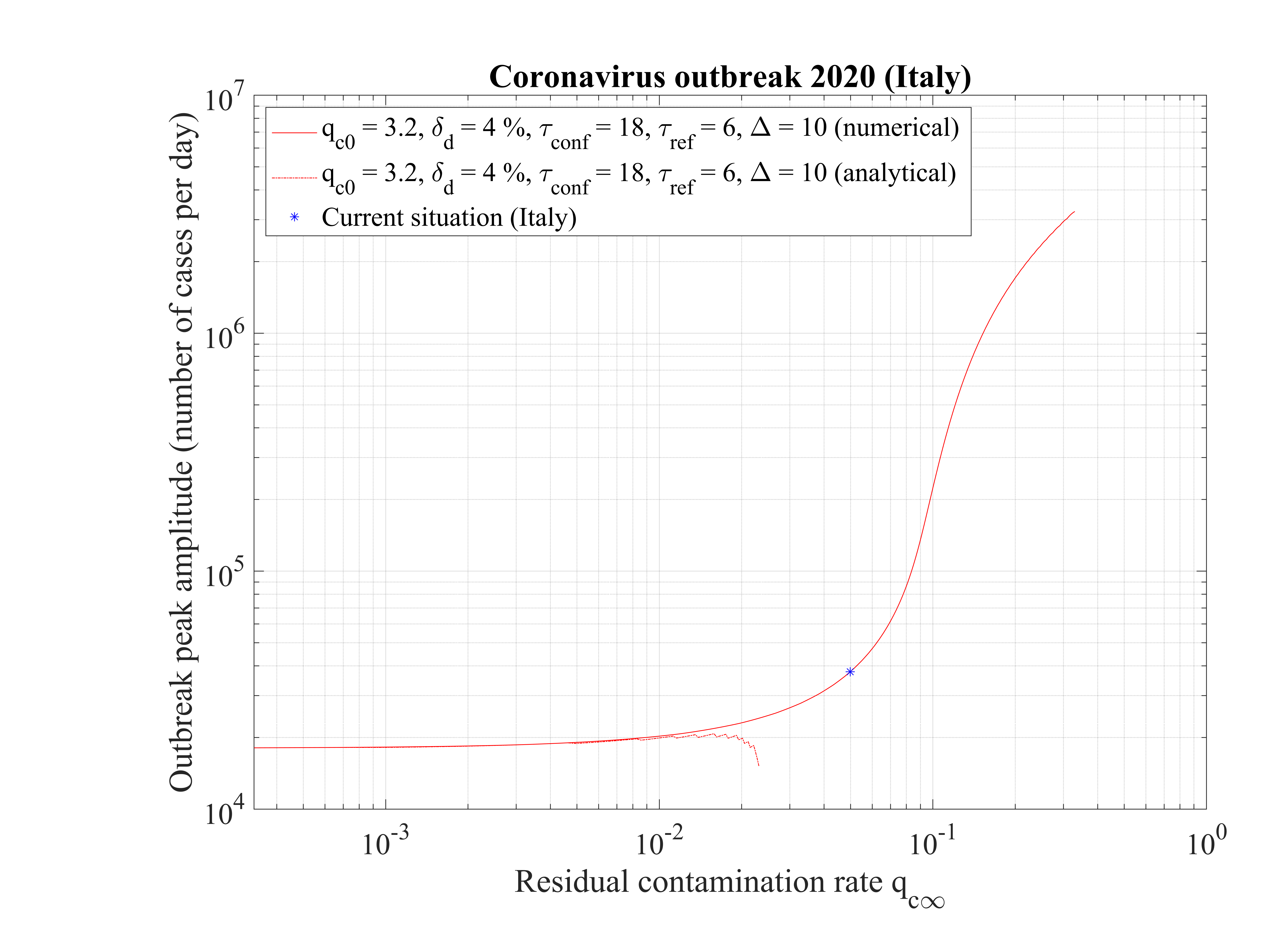
The time at which the outbreak peaks is shown in Fig. 17. It decreases when qc∞ is lowered, but remains almost independent of qc∞, around 45 days, below qc∞ = 0.01. It is 51 for qc∞ = 0.05. The analytical estimate where assumptions holds is also shown and is consistent with observations. Finally, in Fig. 18, the outbreak peak is about 15000 if qc∞ = 0.05.
This analysis shows explicitely the effort that should be done to reach the objectives of a full control and stop of the outbreak.
In this scenario described in Sec. 4.2.1, the reference is the time evolution of the number of deaths Nd and the fatality rate is set to δd = 0.7% based on the analysis of the outbreak in the line cruiser Diamond Princess and in South-Korea. To reproduce the time evolution of Nd, the simulations parameters are : qc0 = 0.44 and qc∞ = 0.32, and the starting day of the outbreak must be shifted a bit earlier by 6 days as compared to the standard case.
As shown in Fig. 19, the actual number of contaminated people is effectively under-estimated, especially after the day 20 corresponding to the change of slope in the official number of positive cases to the coronavirus test (7th of March).
In the low fatality rate scenario, taking δvsv = 2%, gives the correct level of people requiring an active ventilation in continuous health care units, but the slope does match the observation very well as shown in Fig. 20. Indeed, it is overestimated in the early phase of the outbreak, while it is underestimated later. Such a difference must be followed carefully, because it can be a way to decide which one of the two scenarios is the closest to the observations. Again, time dependence analysis is a critical constraint to assess which model of outbreak is the most likely.
In this scenario, the peak of the outbreak is around 62 days after its beginning, and the number of contaminated people will decrease rapidly in 110 days approximately. But, the number of deaths is very high, around 325000, though much lower to the case if nothing is done and the outbreak evolves freely (collective immunity).


The Italy was the first European country to face a major outbreak of the new coronavirus. During about two weeks, the number of cases was almost constant, likely due to travellers coming from infected countries, which were immediately put in quarantine or at hospital. After the 21st February of 2020, the effective outbreak started quickly, and the country is facing a severe outbreak. All data have been obtained the official WHO website.
Since day 0 is chosen to be the starting point of the outbreak, i.e. when the growth
rate of contaminated people starts to become fast. The value qc0 = 3 is taken to fit the
early phase of the outbreak that has a progression like a geometric series as shown in
Fig. 23. It is a very high value as compared to France, which indicates the high level of
the contamination by the virus per day and per person. The Italian government reacts
quite quickly, by setting-up a strong quarantine in concerned areas like in China to fix
the outbreak, and qc falls down rapidly to qc∞ = 0.2, with τref = 3 and △τ = 2.0, as
shown in Fig. 24, and with the evolution of qc
falls down rapidly to qc∞ = 0.2, with τref = 3 and △τ = 2.0, as
shown in Fig. 24, and with the evolution of qc , the cumulative number of sick people is
rather well reproduced, in Fig. 23. Unfortunately, the effort is not enough to contain the
outbreak, and the whole population will be contaminated if nothing is done, i.e. a more
drastic quarantine with transport restrictions is set-up. Even if qc∞ is France and Italy are
close, evolution of the cumulative number of contaminated people is different, because
the initial conditions and the type of reaction to control the outbreak have been rather
different. Nevertheless, with almost same qc∞, the ultimate result is similar: the outbreak is
uncontrolled, like in France, if qc∞ is not drastically lowered, as was reached in China (see Sec.
3.3).
, the cumulative number of sick people is
rather well reproduced, in Fig. 23. Unfortunately, the effort is not enough to contain the
outbreak, and the whole population will be contaminated if nothing is done, i.e. a more
drastic quarantine with transport restrictions is set-up. Even if qc∞ is France and Italy are
close, evolution of the cumulative number of contaminated people is different, because
the initial conditions and the type of reaction to control the outbreak have been rather
different. Nevertheless, with almost same qc∞, the ultimate result is similar: the outbreak is
uncontrolled, like in France, if qc∞ is not drastically lowered, as was reached in China (see Sec.
3.3).
Interestingly, the fatality rate is very high in Italy, δd = 4%, comparable to the value in China (see Sec. 3.3), but more than twice the value observed in France. This difference is unclear, and may result either from a difference in the medication that are given to sick people at hospital, or two types of viruses may circulate, with different level of contamination rate.
As shown in Fig. 25, the italian health care will be rapidly overloaded. At day 16 after the beginning of the outbreak here considered, it is already under high pressure as reported by newspaper.
 than it should be to have continuity at day
18, almost twice more, but after qc∞ is divided by 2.5, which may be the first sign of the
effects of confinement. If this is confirmed, the outbreak should peak at around day 107
(7th of June 2020) with a very slow decrease after. This analysis must be confirmed by
further results in the coming days. The threashold of 10000 deaths is estimated to the
31th of March 2020.
than it should be to have continuity at day
18, almost twice more, but after qc∞ is divided by 2.5, which may be the first sign of the
effects of confinement. If this is confirmed, the outbreak should peak at around day 107
(7th of June 2020) with a very slow decrease after. This analysis must be confirmed by
further results in the coming days. The threashold of 10000 deaths is estimated to the
31th of March 2020.


The non-standard case applied for Italy is interesting when precursors of the outbreak peak is coming. In order to fit the number of deaths with time (cumulative or daily), the two phases must be considered: before the confinament date and after. First, to reproduced the amplitude of the number of deaths, the reference date must be shifted by three days to the 18th of February. The confinement date is of course unchanged. For the first phase, simulation parameters are qc0 = 3.2, τref = 2, △τ = 2 and qc∞ = 0.32. After day 21, they are qc0 = 0.35, τref = 6, △τ = 10 and qc∞ = 0.01. Consequently, the outbreak exhibist a peak, around the 2nd of April (a little bit earlier than for the high fatality rate scenario, 4 days), but the total number of deaths is decreased to 20000 approximately. The end of the outbreak is estimated by end of May, while it is much longer for the high fatality rate scenario (one month more at least). So from the two scenarii, it is possible to estimate the total number of deaths in the interval 20000 - 55000 deaths. The date of the outbreak peak which is robust within 4 days, should occur in the first week of April. All details are available in Figs. 3233.


The outbreak in China started in December 2019, but reports on quantitative data started
the 21st of January 2020. They can obtained from the official WHO website. Since day 0
is unkown, it is adjusted with the qc0 to fit the early phase of the outbreak that has a
progression like a geometric series. It is taken 8 days before the first report, so the 13rd of
January 2020. In order to reproduce the very fast growth rate qc0 = 1.41 is considered and a
good agreement is found with observations (see Fig. 36). The couple made by qc0 and the
initial time has an impact of the saturation of the outbreak, if qc∞ can be low enough.
Thanks to their strong quarantine policy, it falls down to qc∞ = 0.001, with τref = 9 and
△τ = 5.5, as shown in Fig. 37, and with the evolution of qc , the cumulative number of
sick people is rather well reproduced, in particular in the asymptotic phase, though the
exact level is very sensitive to the couple of parameters
, the cumulative number of
sick people is rather well reproduced, in particular in the asymptotic phase, though the
exact level is very sensitive to the couple of parameters  . At the intermediate
phase, at time t = 20, the model seems to overestimate the cumulative number of sick
people, but it can result from the difficulty to rigorously evaluate the effective number of
contaminated people. From the model, China is close to the end of the outbreak, a succes that
is only the consequence of an exceptionnal quarantine. The last day of the outbreak is
54.
. At the intermediate
phase, at time t = 20, the model seems to overestimate the cumulative number of sick
people, but it can result from the difficulty to rigorously evaluate the effective number of
contaminated people. From the model, China is close to the end of the outbreak, a succes that
is only the consequence of an exceptionnal quarantine. The last day of the outbreak is
54.
In order to reproduce the cumulative number of people who died from the virus, a mortility of 4% must be applied, close to the value for Italy. Seems to be much larger than in France, which is only 1.5%. This may result from the use of advanced medication, still an open question. Finally the calculated daily number of contaminated people, and those very sick requiring or not an artificial ventilation is given in Fig. 38.


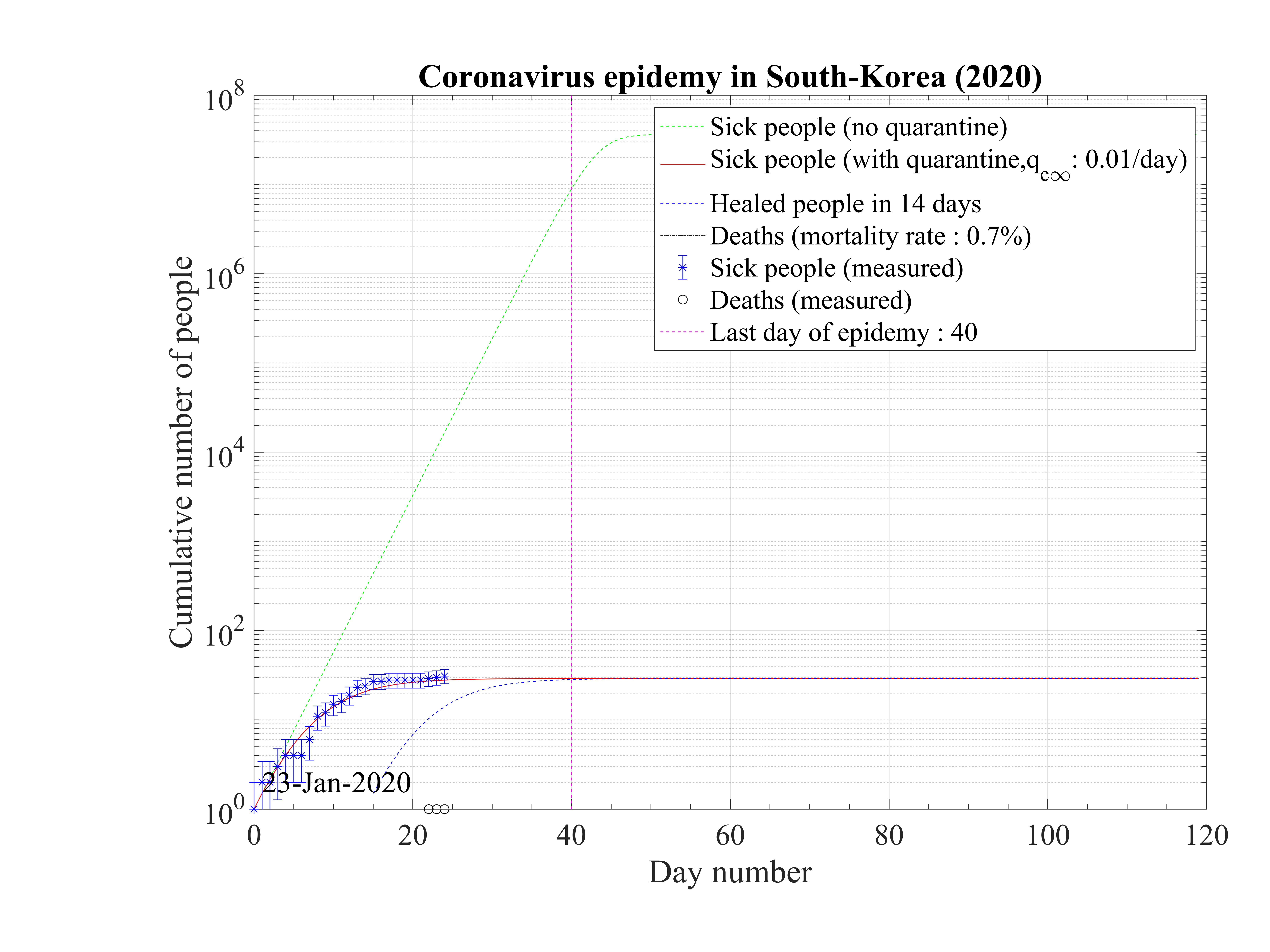
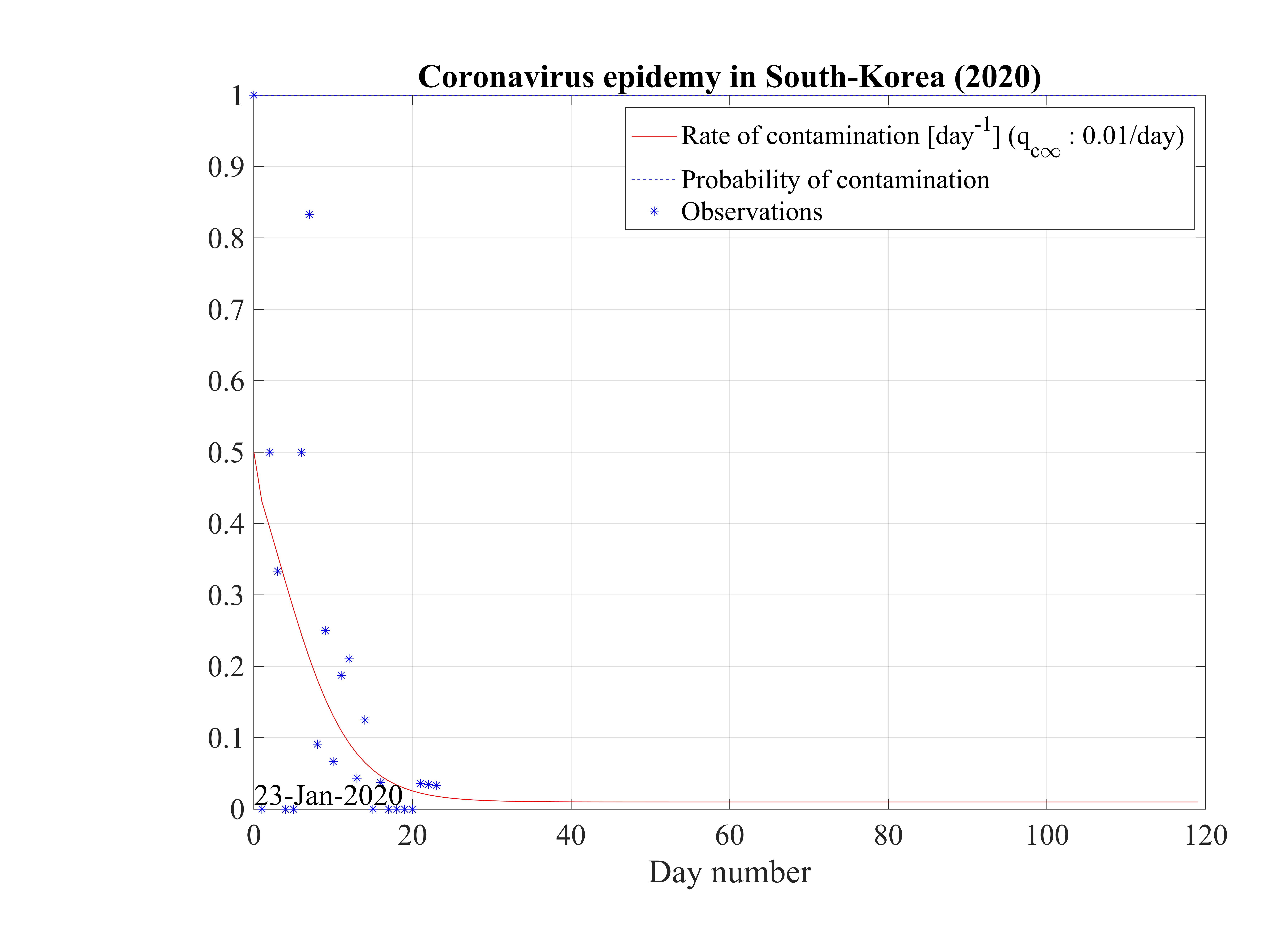
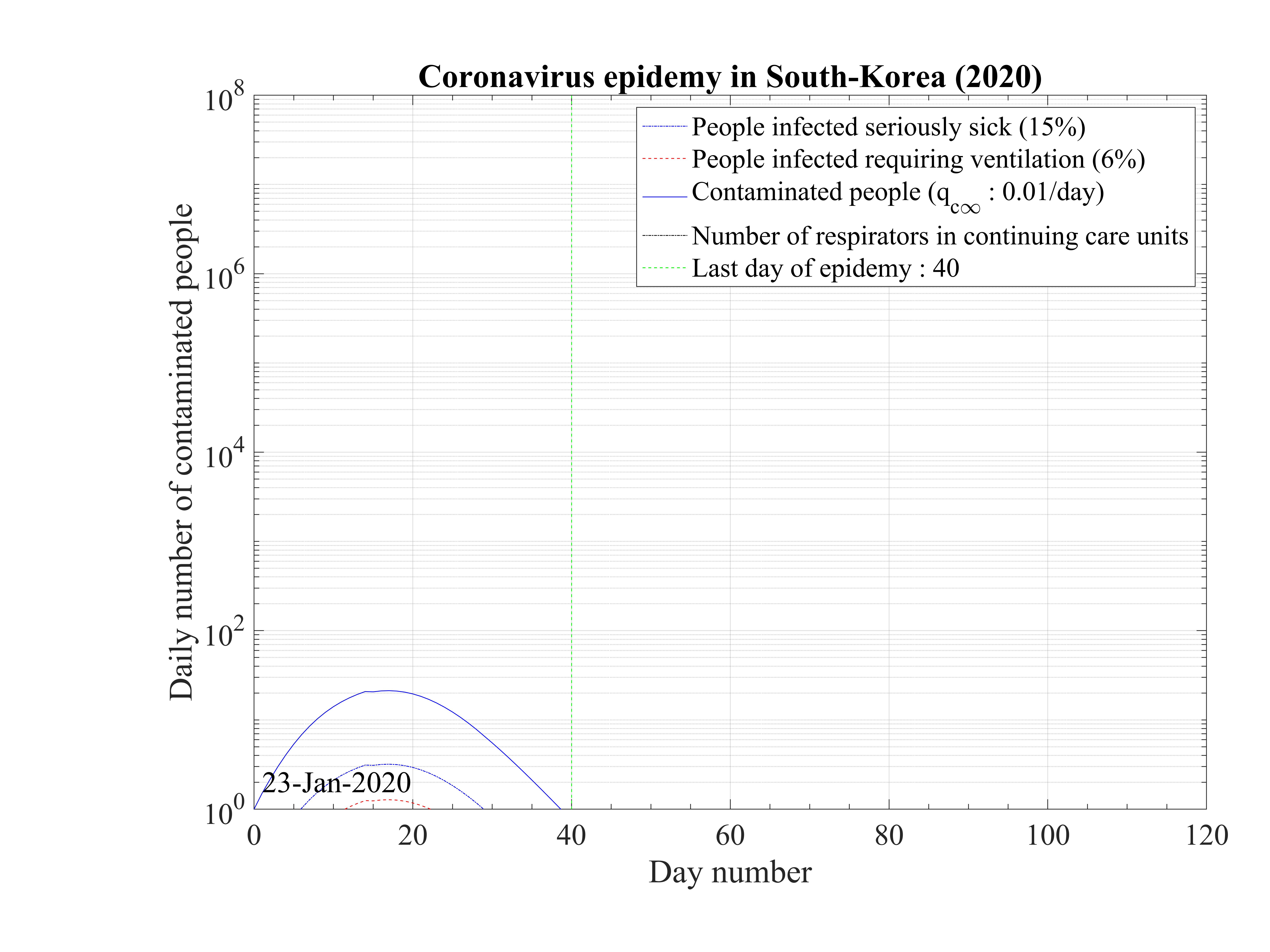
South-Korea was one of the first country except China facing the coronavirus outbreak. Data can be obtained here. It is characterized by two steps as shown in Fig. 46. The first case was identified the 20th of January, and the epidemy was rising exponentialy until the 18th of February, giving up to 31 cases up to that time with a single death. As shown in Fig. 43, the outbreak was rapidly controlled, but the initial growth rate was fairly low and falls down rapidly as shown in Fig. 44. Simulations parameters are qc0 = 0.5, qc∞ = 0.01, with τref = 4 and △τ = 4.5, and the end of the outbreak is expected after 40 days (see Fig. 45)
Unfortunately, after a member of the Shincheonji religious organisation was detected as
contaminated during a large meeting, the growth rate of the number of contaminated
people was suddenly explosive, and the governement reacted immediately by setting up
a strong quarantine. This led to a quick decrease of the contamnation rate qc and a
fast stabilisation of the outbreak that is back under control with qc∞ = 0.01 as shown
in Fig. 47. This highlight the importance to cancel all meetings with a large number of
participants, and also the fast that since most of the population is not immunited against
the virus, the outbreak can restart almost immediately. Therefore, even if the outbreak
ends, a continuous control is necessary with fast reaction to avoid an avalanche effect.
As shown in Fig. 46 the time evolution of the epidemy is well reproduced, as well as the
number of deaths. New simulations parameters after day 24 are qc0 = 1.05, qc∞ = 0.01, with
τref = 4 + 24 = 28 and △τ = 4.5, indicating that it was a bit more difficult to control the
second rise of the outbreak. Nevertheless, Korean authorities were able return back to a
controlable situationn, but the outbreak is postponed and last at around 68 days after
the initial reference time here considered, the 23th of January, so by end of March (Fig.
48)
and a
fast stabilisation of the outbreak that is back under control with qc∞ = 0.01 as shown
in Fig. 47. This highlight the importance to cancel all meetings with a large number of
participants, and also the fast that since most of the population is not immunited against
the virus, the outbreak can restart almost immediately. Therefore, even if the outbreak
ends, a continuous control is necessary with fast reaction to avoid an avalanche effect.
As shown in Fig. 46 the time evolution of the epidemy is well reproduced, as well as the
number of deaths. New simulations parameters after day 24 are qc0 = 1.05, qc∞ = 0.01, with
τref = 4 + 24 = 28 and △τ = 4.5, indicating that it was a bit more difficult to control the
second rise of the outbreak. Nevertheless, Korean authorities were able return back to a
controlable situationn, but the outbreak is postponed and last at around 68 days after
the initial reference time here considered, the 23th of January, so by end of March (Fig.
48)
Suprinzigly, the fatality rate is much lower, about δd = 0.7%, while it may be about 3 - 4% transiently, though statistical uncertainty is very large. Nevertheless, the drop of the mortality may indicate that the quarantine has led to isolate the most fragile population to the virus.

The coronavirus outbreak is major issue in Iran. From data that can be obtained here. Afster a fast raise of the outbreak, first stabilization after about two weeks. Before, no control of the outbreak was observed, since the data follows the curve without quarantine. The values are quite usual, qc0 = 0.75, △τ = 2.0, τref = 2 and qc∞ = 0.1, but τref = 15 which means that the authorities reacted late, explaining why the number of confirmed cases is so large. Neverthless, the quarantine-like in Iran was quite effective, since qc∞ = 0.1, quite low as compared to European coutries and USA, leading to a stabilization of the growth rate of the number of confirmed caes, but not a control of the outbreak.
In the early phase of the outbreak, the number of deaths was very large, and this is not well explained, except if the initial numbers are wrong, and the outbreak started well before as it was claimed (like in South Korea, with a two steps evolution). At the date of the 11th of March, the fatality rate reaches δd = 3.0%, consistently with other countries. The small rise observed after the 9th of March may result from a restart of the outbreak, that is not correctly followed by the counting of the confirmed cases.


In Switzerland, the outbreak starts to grow quickly too with qc0 = 0.75. Status of the outbreak may be found here. The simulation parameters are τref = 10 and △τ = 2.0, with qc∞ = 0.15, which leads to a rapid growth rate of the number of cases. Nevertheless, the outbreak in not controlled at the date of the 6th of March 2020. The mortality rate is estimated to δd = 0.4%, much lower than for France, by a factor 4 at least, since just one death is officaly reported the 9th of February, and two for the 11th of March. Results are shown in Figs. 54, 55 and 56. Regarding the time evolution of the number of confirmed cases, there is large uncertainty on qc∞.


The outbreak starts to be quite aggressive in United-States of America. Several states have declared the emergency state. Nevertheless, the domestic outbreak by local spread of the virus seems to have started at the date of 19th of Febrary, as indicated by the two steps evolution of the number of the confirmed cases in Fig. 59. For the second rise, simulation parameters are qc0 = 0.4, with τref = 7 and △τ = 2.0. It is a rather slow growth rate, perhaps because the country was already prepared to face the outbreak. Nevertheless, with qc∞ = 0.4, the outbreak is not controlled. Note that qc0 = 0.4 is rather low as compared to other countries, and this may result from the fact that the population density is lower in USA than in other countries, so the probability to contaminate somebody is lower.


The case of Spain is very similar to USA.The outbreak started effectively the 23th of February, and the evolution is well modeled by following parameters: qc0 = 1.0, qc∞ = 0.25, with τref = 7 and △τ = 2.0. There is no specificity of Spain as compared to other countries. The initial phase of the outbreak seems to have been slightly more agressive, but the contimation rates felt down rapidly to standard European levels, ranging between qc∞ = 0.20 - 0.30. Obviously, the outbreak is not under control at this stage. All results can been seen in Figs. 63, 64 and 65.


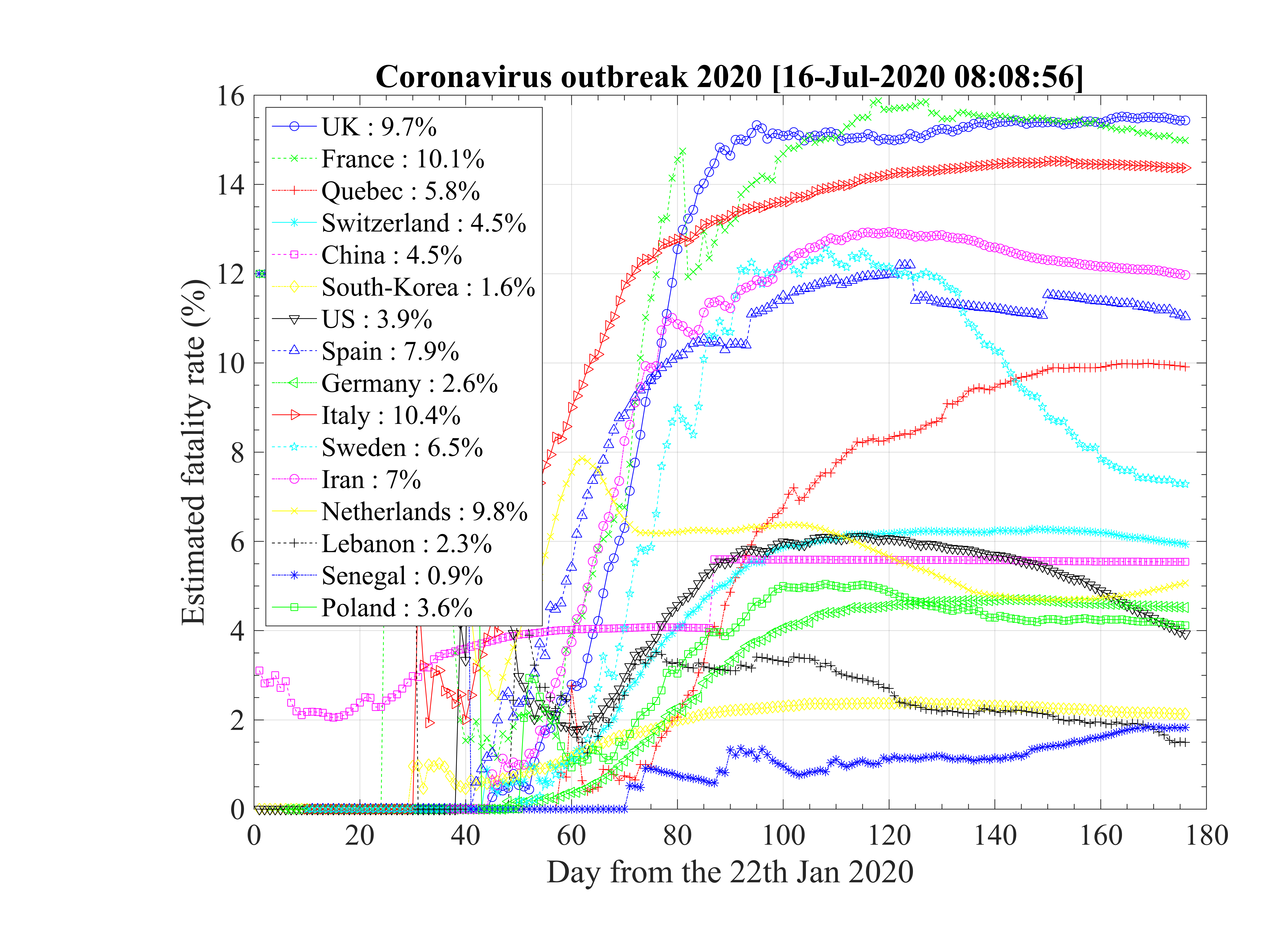
Global data analysis gives interesting trends about the outbreak, and how it has been managed by various countries. All main parameters are summarized in Table 1. Those who are able to reach a residual contamination rate qc∞ < 0.05 by quarantine or other techniques have a large chance to control the outbreak in a finite time (less than four months) with a small number of people contaminated, and also, by consequence a small number of deaths. This concerns China and South-Korea at present time. Iran seems to be in the good direction though it has to be confirmed. All other studied countries have an uncontrolled evolution of the outbreak, despite what is claimed in the media, with the actual data. This may change, but it has to be demonstrated !
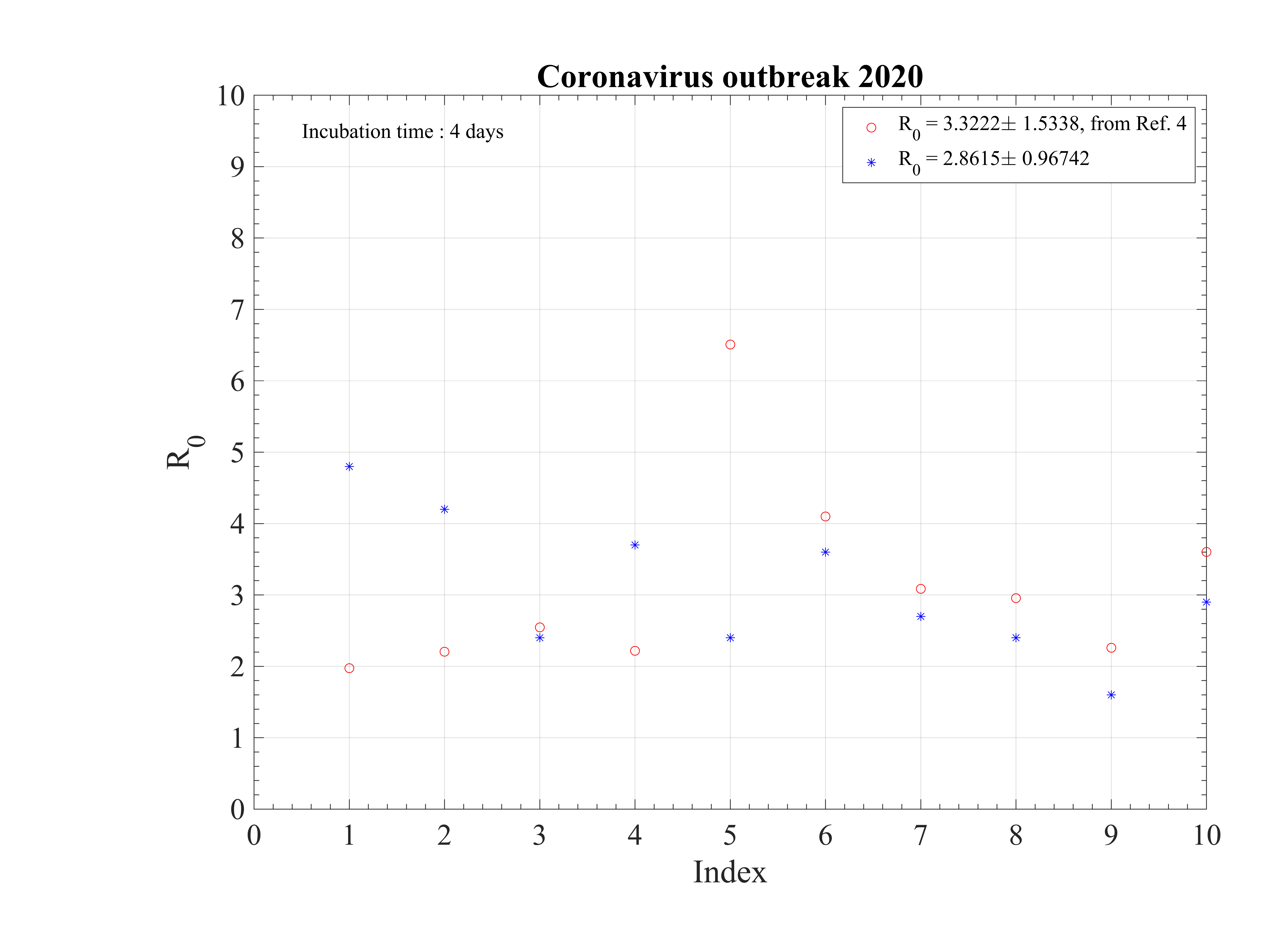
The initial contamination rate in most countries is similar, thanks to the difficulty to get accurate numbers and the statistical uncertainty (low level of number of confirmed cases in some countries). Its mean value is c0 ≃ 1 approximately, which means that a single person that is contaminated can contaminate about one person per day approximately. This corresponds to a R0 ≃ 3.4±0.9, excluding Italy, with the incubation time of τi = 4 days that is here considered. It can be compared to first estimations using different type of codes, as shown in Fig. 92 [4]. Of course, the estimation of R0 is highly sensitive to the incubation time τi. If it is lowered, a lower R0 is found. There is a rather large controversy in the recent litterature on this point [4, 5, 6].
The seasonal flue is much less (five times, which is the reason of the danger of this outbreak) and it is about 2 times larger than the Spanish flue [7]. It remains nevertheless three times less than the measles R0 = 12 - 18 (Source Wikipedia). After, thanks to the quarantine or the natural reaction of the population becoming cautious, it drops down quite rapidly to lower values. The delay τref is rather similar for all countries, except for Italy, that was fast despite the bad actual situation, and Iran which was very late. The rate of decrease is similar is most countries, but twice lower in Asia. This latest parameter indicates the effectiveness of the reduction of the contamination rate.
As shown Table 1, the fatality rate never exceeds δd < 4%, though a degradation seems to occur Italy after the 9th of March 2020. But this may arise from a bad evaluation of the confirmed cases. In Iran, after an initial fatality rate that seems totally over-estimated, it reaches the standard level, about δd = 3.0%. This evolution is clearly seen for Spain, Italy.
It is common to hear that official figures are false or biased. This is unlikely, as for some countries, since different sources give same results. In addition, simulation parameters are rather similar, whatever the country. The consistency between the number of confirmed cases and deaths, whose ratio in addition is independent of time is also an indication of the robustness of the data. Nevertheless, different policies exist between countries, as well as techniques to identify unambiguously people that are contaminated or died from coronavirus. The error bars on data is certainly much larger than the level from Poisson’s statistics, is is related to the test methods uncertainty to identified people that are effectively infected by the coronavirus. Details mays be obtained here.
From the determination of R0 it is possible to estimate the fraction of the population that must be immunited to stop the outbreak. It can be done by vaccine or naturally. Data using Eq. 11 are given in Table 1. It is interesting to not that this fraction is 33% for the seasonal flu, and 95% for the measles, thanks to their respective basic reproductive number.
| R0 | f [%] | qc0 | qc∞ | τref | △τ | δd | Control | |
| China | 4.8 | 79 | 1.2 | 0.05 | 2 | 8 | 4 | Yes |
| South-Korea | 4.2 | 76 | 1.05 | 0.01 | 4 + 24 | 4.5 | 0.7 | Yes |
| Italy | 2.4 | 66 | 0.6 | 0.047 | 23 | 10 | 4.0 | Yes |
| Iran | 3.7 | 73 | 0.93 | 0.05 | 4 | 10 | 3.0 | Yes |
| Spain | 2.4 | 66 | 0.6 | 0.045 | 27 | 6 | 2.5 | Yes |
| Netherlands | 3.6 | 72 | 0.91 | 0.06 | 6 | 11 | 0.5 | Yes |
| France | 2.7 | 62 | 0.67 | 0.02 | 3 | 18 | 2.5 | Yes |
| Switzerland | 2.4 | 58 | 0.6 | 0.05 | 4 | 15 | 2.0 | Soon |
| USA | 1.6 | 36 | 0.385 | 0.01 | 33+17 | 7 | 1.5 | Soon |
| Germany | 2.9 | 66 | 0.73 | 0.06 | 2+30 | 16 | 0.1 | Soon |
| United-Kingdom | 2.1 | 51 | 0.51 | 0.03 | 33+22 | 11 | 1.0 | Soon |
| Sweden | 2.8 | 64 | 0.7 | 0.11 | 2 | 14 | 0.3 | Soon |
| Qu´ebec (Canada) | 1.6 | 37 | 0.4 | 0.05 | 32 | 6 | 1.0 | No |
As shown in the calculations, the mortality rate is varying significantly between countries (see Fig. 93 ), in particular within Europe where health care systems are similar. The increase of δd with time is a sign that the statistics of confirmed cases is becoming progressively wrong as the outbreak develops. This justify why δd of the cruise liner Diamond-Princess is likely the only robust value and the two scenarii that will be discussed below.
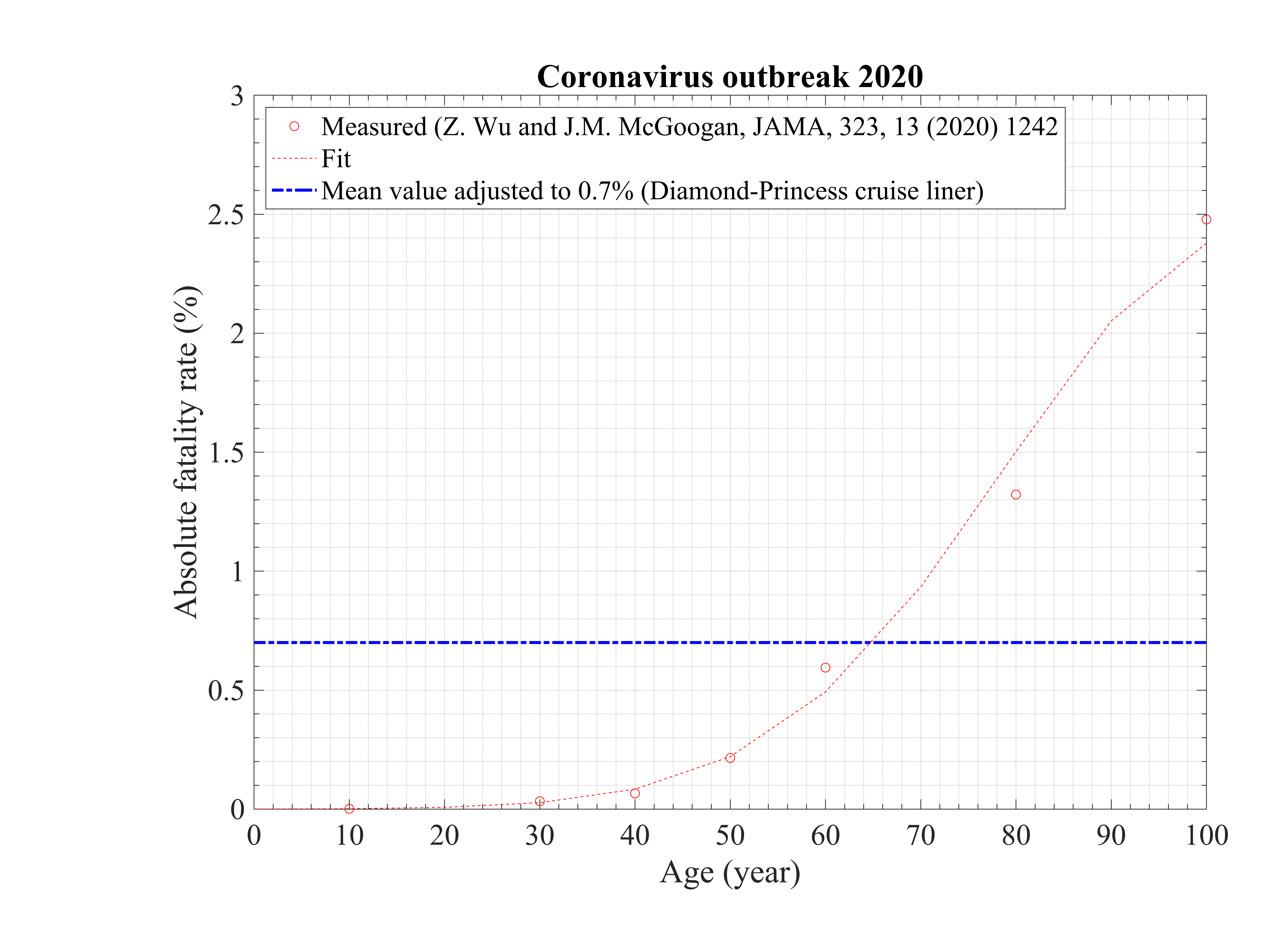
It is known that old people are much subject to death than young people, by more than two orders of a magnitude from a Chinese study based on 45000 persons. According to this study, the mean mortality rate is between 2.3%, but 0% for children les than 10 years old, 0.2% like the flu (twice more precisely) for people less than 39 years old, 0.4% for the forties, 1.3% between 50 - 59 years old, 3.6% for the sixties, and 8.0% for the for octogenarians and beyond likely 15.0% (see Fig. 94) [6]. In addition, two third of the deaths arised from men, and this pulmonary fragility is likely linked to tobacco consumption
. The role of co-morbidity may play likely a very significant contribution to the fatality rate. Indeed, the case of the cruise liner Diamond Princess is enlightening on this point of view. With about 4000 passengers onboard, 705 (after landing a bit less, with 696 confirmed contaminated people) of them where unambiguously diagnosed as contaminated, and only 7 deaths have been recorded. This corresponds to δd = 1.0%, close to the value in South-Korea (at the beginning of the outbreak), where broad test campaigns have been carried out. Since this population was rather old, and one can suppose that it was in rather good health to do the trip, δd is much lower than standard estimates in many countries, and disagree with analysis that claims a strong age-dependence of the fatality rate. Therefore, a possible interpretation as follow: δd is around 1.0% for people in good health, what ever the age above 50 years old (less for younger people), and larger mean δd may arise from a underestimate of the actual number of people contaminated (sampling is done more than and full effective measurement), except in South-Korea, together with the age dependence of the fatality due to co-morbidity. So already weak people suffering from serious illness are much more sensitive to the effect of the virus. an indication of the role played by co-morbidity is the fact that men and women in China are almost equally contaminated (slightly more men), but 2∕3 of very sick people dying are men. It may be the consequence of the poor lung condition of Chinese men who are known to smoke a lot.
This interpretation leads to to approach :
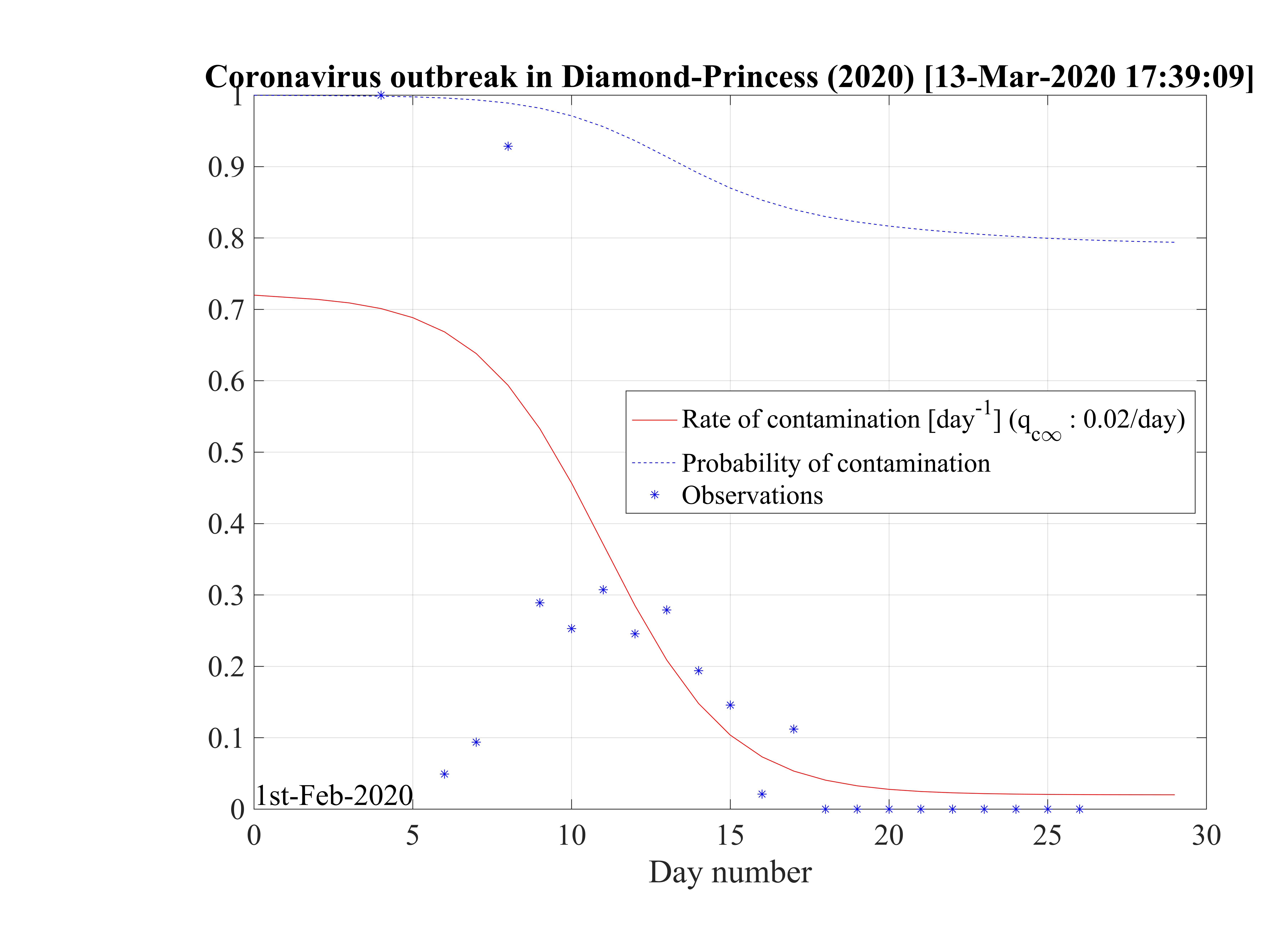
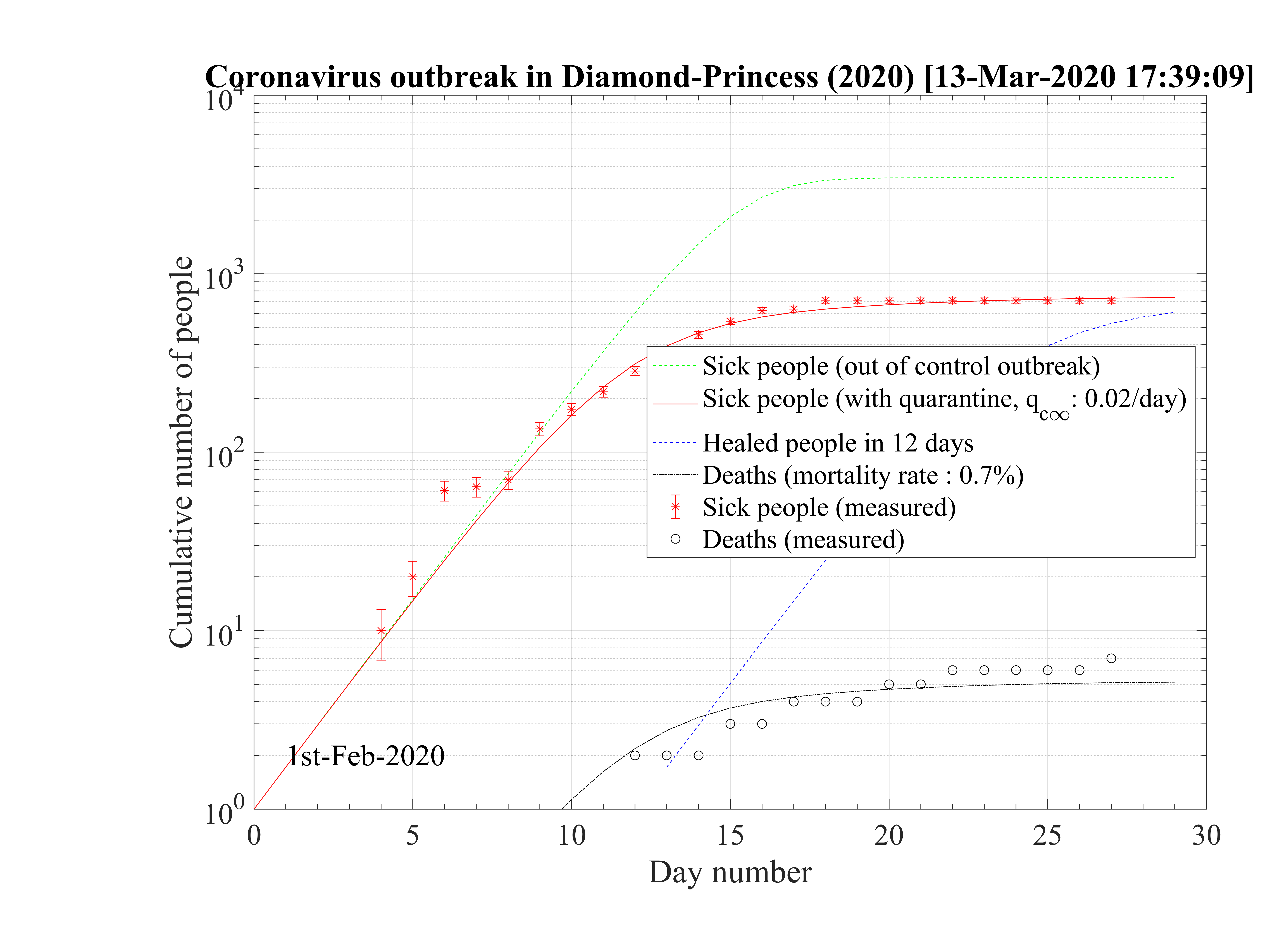
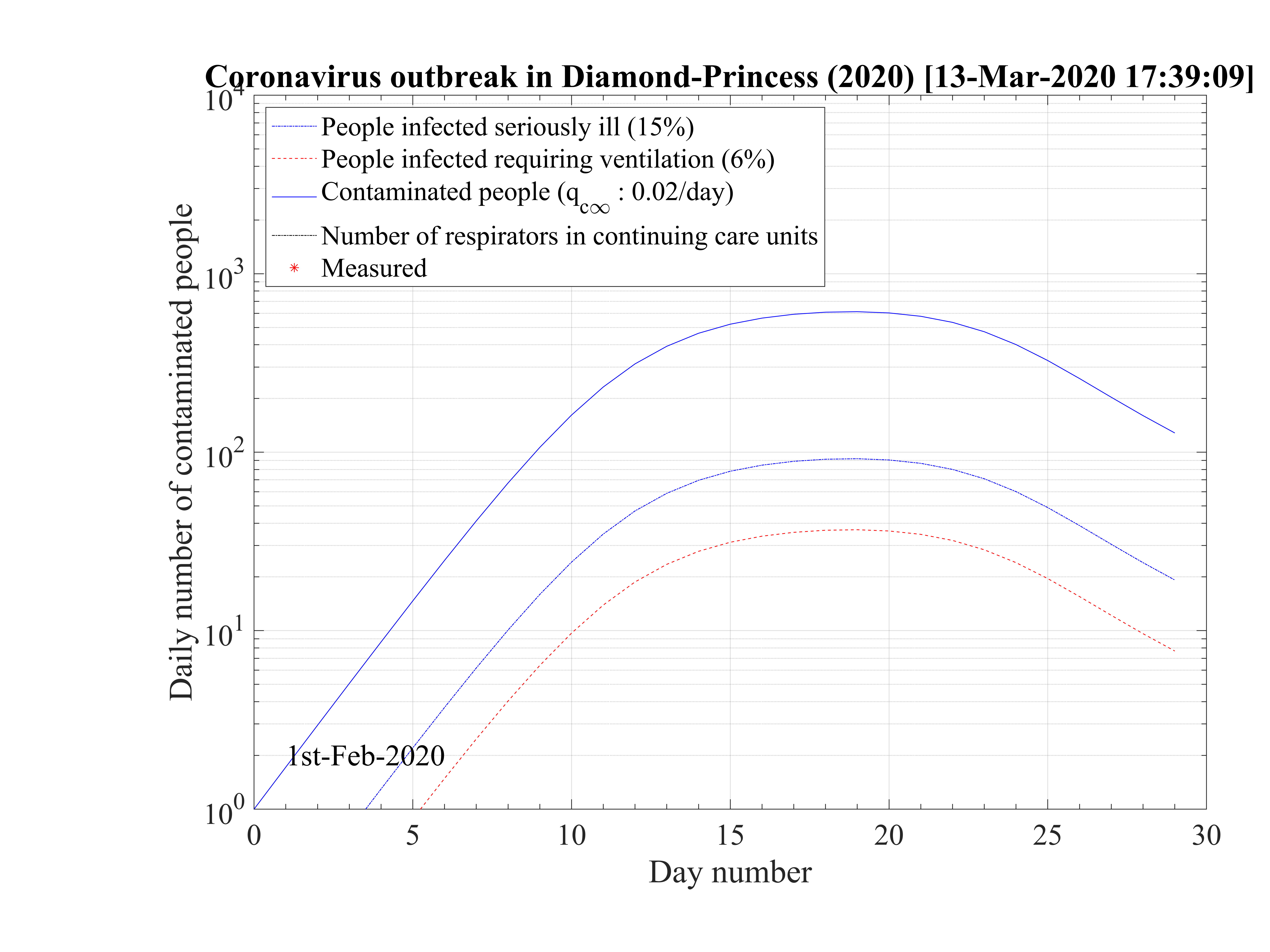
The cruise liner Diamond Princess has been contaminated around the 1st of February 2020, and the outbreak spreads rapidly onboard. It was placed in a strong quarantine near Yokohama in Japan, and all passengers where forced to stay in their cabins during more than two weeks approximately. The 3711 passengers + crew where all tested against the contamination by the coronavirus, and ultimately, 705 where diagnosed positive (after landing a bit less, with 696 confirmed contaminated people). Seven people died, so δd = 1.0%. A shown in Fig. 95 the outbrak started very quickly, like in countries, but thanks to the strict quarantine, it slowed down rapidly and the qc∞ felt down to 0.02, like in countries which succeeding in the control of the outbreak. The outbreak was controled in the cruise liner in 26 days. The outbreak never reach the 60% saturation level, and without quarantine, 34 passengers would have died. The reservoir effect, though significant, remains less than 20%, thanks to the effectiveness of the quarantine (Fig. 96). Simulations parameters are: qc0 = 0.72, qc∞ = 0.02, with τref = 12 and △τ = 2.0. Since τref is large, it means that the reaction of the crew was rather late, concerning the danger of the outbreak inboard. The daily number of sick people is given in Fig. 97.
This case is particularly interesting because it shows unambiguously the effectiveness of a strict quarantine. The residual contamination rate must be lowered less than qc∞ = 0.02 to successfuly control and stop the outbreak. This result is fully consistent with calculations for China and South-Korea. None of the other countries have reach this level, and therefore will control the outbreak at the date of the 14th of March. Moreover, the air-conditioning system has not spread the virus, otherwise the outbreak would have been out of control in this closed volume. This is an important result, that clearly highlight the importance of the close contacts for oral contamination or possibly the contamination by skin contacts. Wearing gloves can be an important test to prevent the spread of the virus, given that it seems to last a long time on surfaces.
The low fatality rate δd = 0.7% while the mean age of the passengers was above 50 years old, but in rather good health to do the trip is a sign that co-morbidity may be the reason for strong age dependence of the fatality rate, as suggested by the Chinese study. This number is closed to the value estimated in South-Korea, which performed a broad control of its population and not a random sampling that is likely done in many countries, by failure of the health care system, or by lack of available tests.
From this analysis, and South-Korea data, a low fatality rate scenario is described as indicated in Sec. 4.2.1, and will be applied to all countries suffering the outbreak that have been studied. From the high and low fataility rate scenarii, it will give some reasonable limits on the development of the outbreak, on its end date and on the ultimate total number of deaths that is expected.
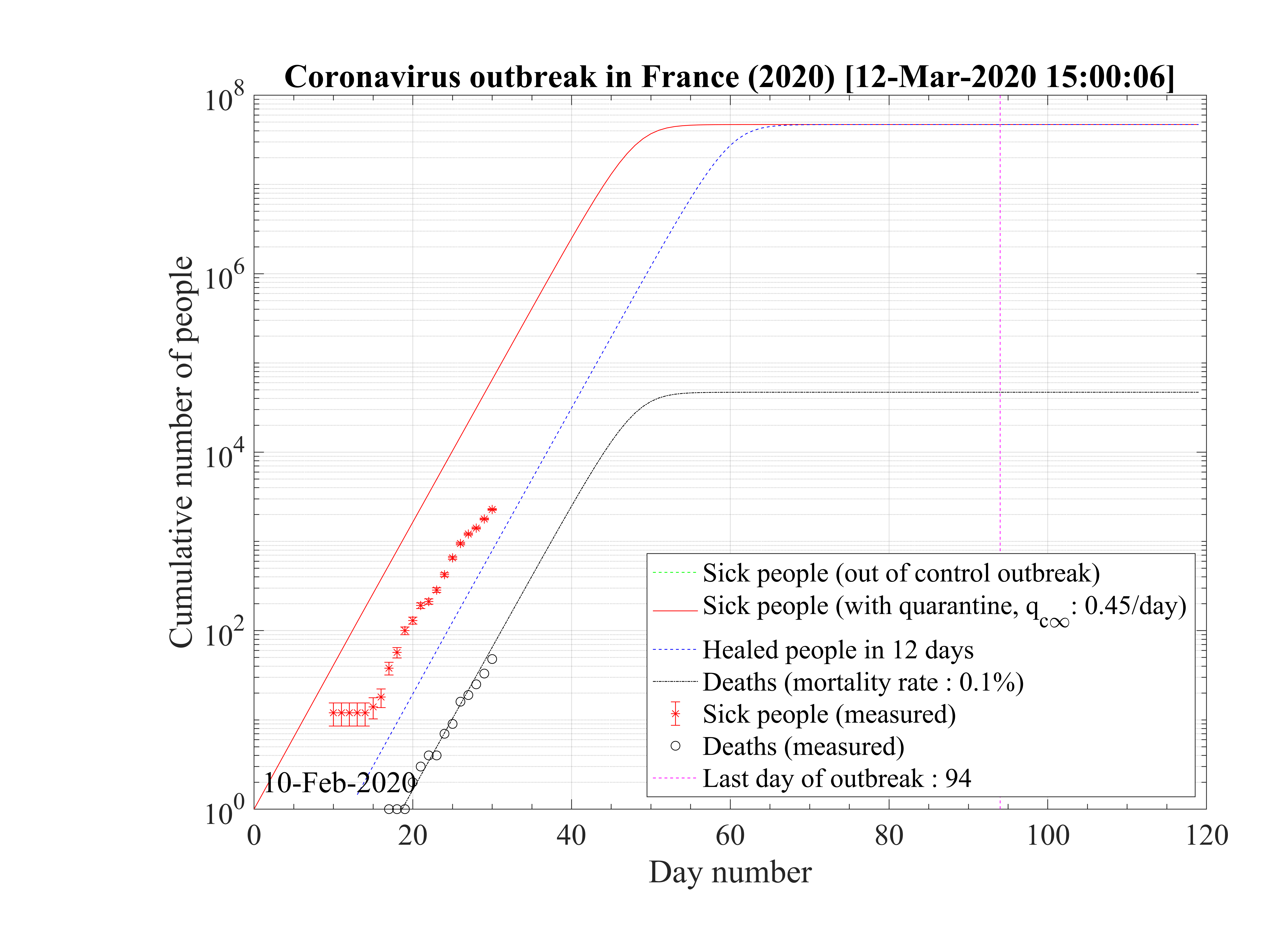
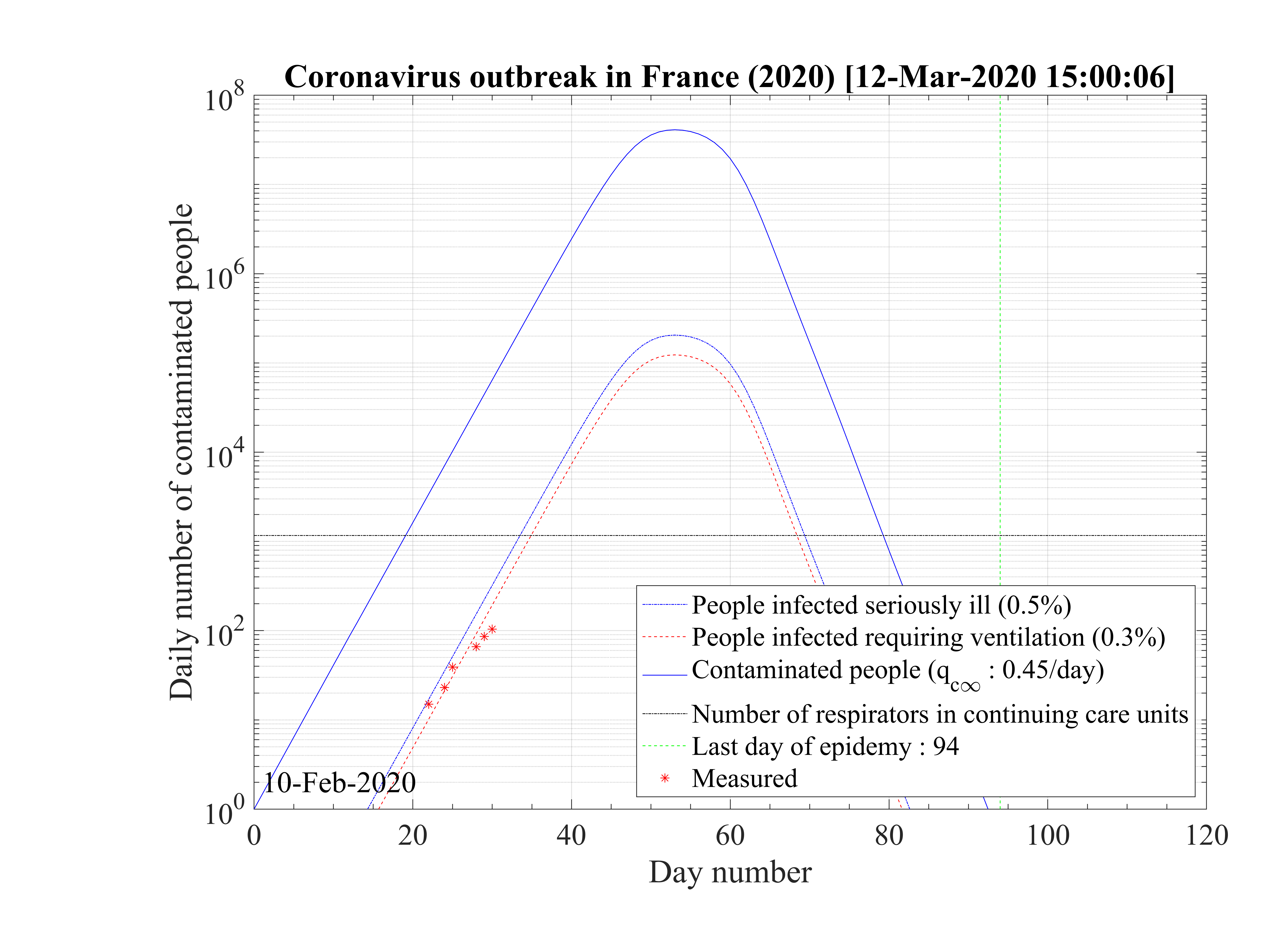
The possibility that the number of contaminated persons could have been very strongly
underestimated is studied. In order to reproduce the outbreak, and considering that only the absolute
number of deaths matters (low fatality rate scenario), with the fatality rate of the seasonal flu,
δd = 0.1%, and considering in addition that the contamination rate is so high that the outbreak is
totally out of control since the beginning, one must consider the following simulations
parameters : qc0 = qc∞ = 0.45 to reproduce observations as shown in Fig.98. In that case the
domestic outbreak should have started 10 days before the bifurcation of the number of official
contaminated cases, at around the 10th of February 2020. If such a situation is true, it means
that all the french population will become immunited in almost 40 days, and after 53
days the outbreak should naturally slow down, as shown in Fig.99 and a decrease of the
number of daily deaths should be also observed. The outbreak would have led to up to 47000
deaths in this simulation, which is quite significant as compared to the seasonal flue but
much less than the standard approach, based on both numbers: contaminated people and
deaths. The difference with the seasonal flu arises from the rate of contamination that
must be much higher for the coronavirus to reproduce the growth rate of the number of
deaths. Interestingly, the number of people which require active ventilation in continuous
health care units must be lowered to δvsv = 0.6% in this case to be approximately to the
level of actual observations. But thanks to the simulation, this number should break very
quickly the threshold of the number of available respirators, thanks to the large rate of
contamination to reproduce the number of deaths (at day 34, so at the date of the 15th of
March 2020). The slope in time is not well reproduced, since calculated Nvsv must
grow less quickly than observations. At the date of the 11th of March, 2281 confirmed
cases have been officialy reported, while the effective number of cases should be more
than 65000 ! A considerable difference effectively, but noboday can confirm this hidden
number.
must
grow less quickly than observations. At the date of the 11th of March, 2281 confirmed
cases have been officialy reported, while the effective number of cases should be more
than 65000 ! A considerable difference effectively, but noboday can confirm this hidden
number.
In anycase, whatever the approach, the overload of the hospitals will come soon and even sooner if the number of contaminated people is deeply underestimated, considering the COVID-19 outbreak like a standard flu outbreak.
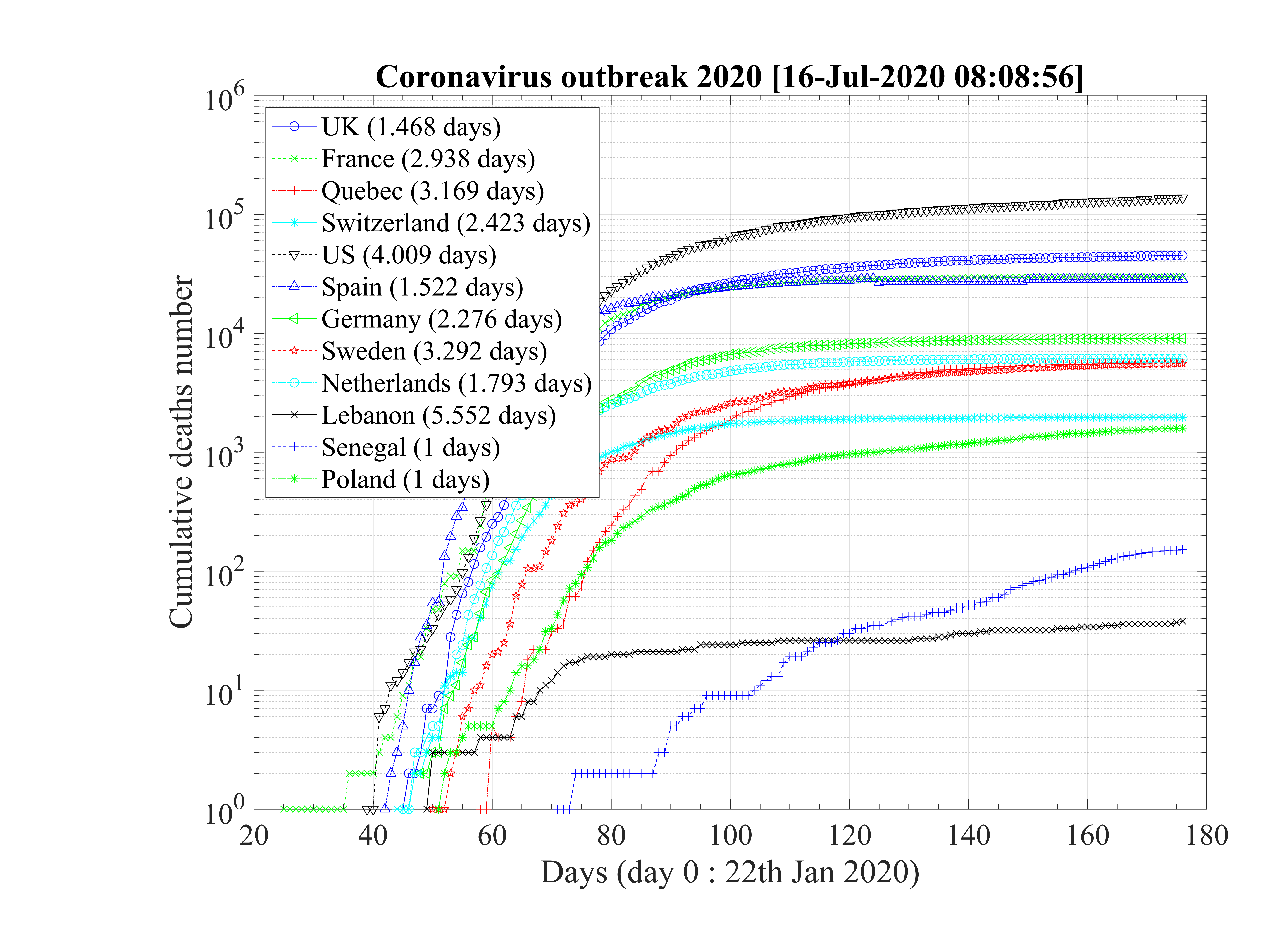
Statistical analysis of the number of deaths in the studied countries has been carried out to test if the time sequence for each country is similar or not. As shown in Fig. 100 for the countries which do not exhibit a soon occurence of an outbreak peak, the exponential growth rates are very similar, and the mean value is about τD = 2.74 ± 0.52 days. When data of these countries are normalized to the highest value (Spain, the 28th ofMarch), the exponential growth rates are very similar too. From the fit of all data, the doubling time is about τD = 2.87 days.
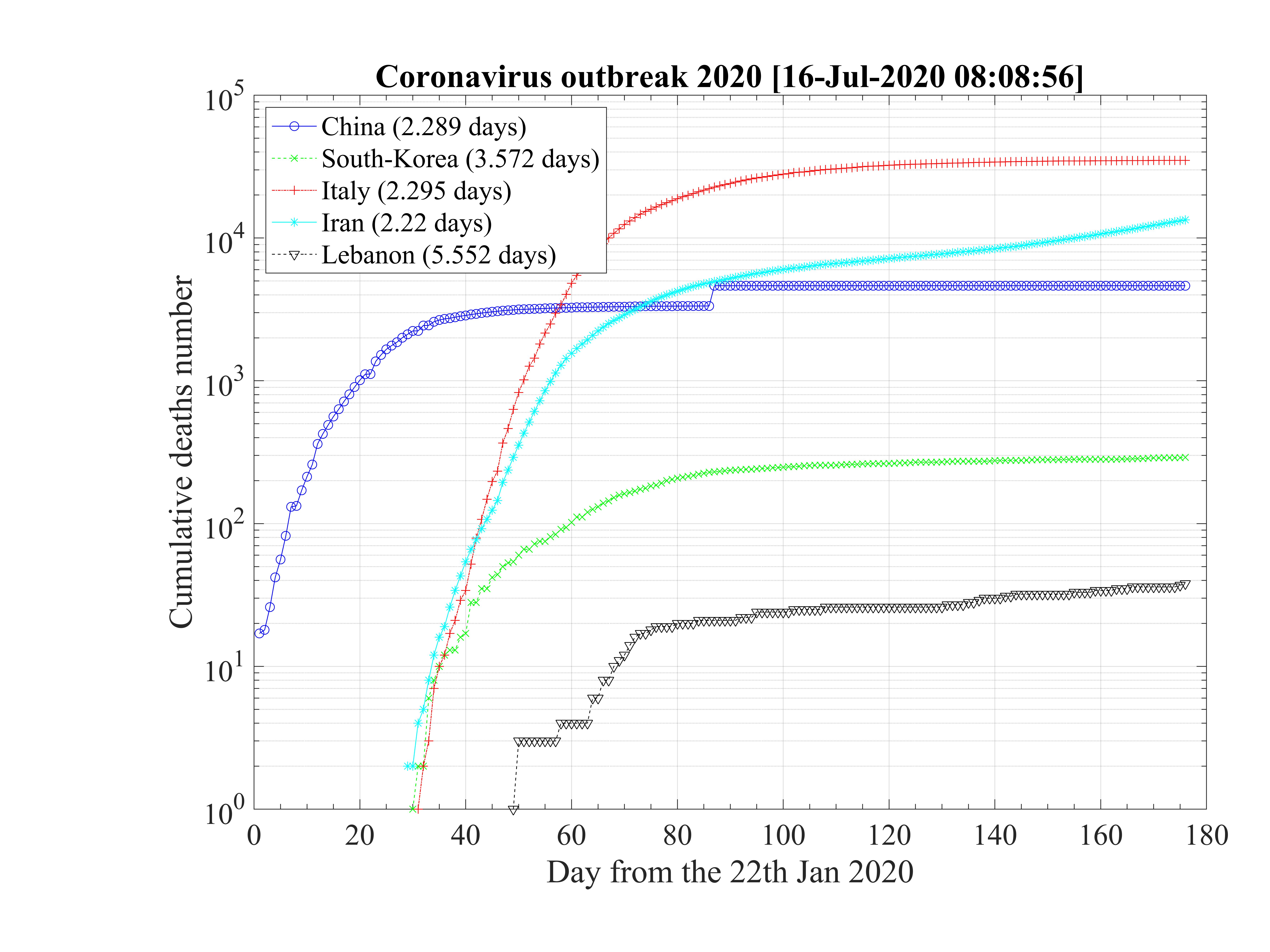
For countries that have past the outbreak peak, or are close to it, as shown in Fig. 101, the doubling time is estimated from the first few days. The mean doubling time is shorter if 6 days are considered, τD = 1.98 ± 0.21, but compatible to previous estimations within error bars. When 8 days are onsidered, it becomes τD = 2.59 ± 0.65 days.
So, even of the fatality rates vary on two orders of magnitude, the time suite of data concerning the cumultaive number of deaths is totaly consistent for all countries. The reference is about the doubling time is τD = 2.69 ± 0.54 days.
The mean contamination rate from time evoluton of the cumulative number of deaths may be easily obtained in the approximate limit
ln = ln = ln
|
or
 | (54) |
or
 | (55) |
such that
 | (56) |
If τD ≥ 1, qc0 ≤ 1, and for τD = 2, qc0 ≃ 0.41. The reproduction factor is then
 | (57) |
From the cumulative number of deaths, and taking an averaged value τi = 7.0 days from study concerning travellers of Wuhan, Rc ≃ 2.13 for τD ≃ 2.6,since Δt = 1 day. This value is lower than the basic reproduction factor Ro ≃ 2.78 determined from the early phase of the outbreak, using the cumulative number of contaminated people, but there is large uncertainties from country to country. As shown in the detailed time evolutions, the fast initial rise is usually followed rapidly by slower rate, consistent with the cumulative number of deaths, which becomes more observable later. The value of Rc is larger than 1, so consistently, the epidemy is still active in many countries, expect China, South-Korea, Italy and Iran, at the 28th of March. Its value corresponds to qc∞ ≃ 0.26. To control the outbreak, qc∞ ≪ 0.25, and a value of qc∞ ≤ 0.05 must be targeted.
The question of the dynamics of the outbreak is a major issue for an appropriate policy. It can be seen that countries or regions (or cities) with dense populations are the most affected. This is obvious because the probability of interaction between people is higher. The high density case studied are boats (Charles-de-Gaulle aircraft carrier, and Diamond-Princess cruise liner). For comparison in Paris, the density is 12,000 inhabitants / km2. On a boat like the Charles-de-Gaulle, which is 245 m long and 65 m wide, considering 3 bridges, the population density is 1,700 * 1,000,000 / 245/65/3 = 35000 people / km2! No wonder the epidemic is exploding. By way of comparison, in Marseille city, the population density is 3500 inhabitants / km2, therefore much less. In Wuhan, it is 5800 inhabitants / km2 (less than in Paris!), And in New York it reaches 7,100 inhabitants / km2. In Dakar, Senegal, it is like that of Paris, 12,000 inhabitants / km2, while there are only very few deaths ... In Africa, with significant disparities, the population density is generally low, 40 inhabitants / km2 (Europe 73 inhabitants / km2, United States 33 inhabitants / km2, China 148 inhabitants / km2, and India 395 inhabitants / km2) except in Nigeria (Lagos in particular with 21,300 inhabitants / km2). And it is in Lagos capital in Nigeria that there are the most cases! So if population density is an important factor, it is in localized areas where density is extreme that the outbreak spreads the fastest.
However, the question of fatality, which is the essential psychological factor in any outbreak, does not exactly follow the density of the population. In addition the fatality linked to 100% COVID-19 may be subject to discussion, and it is very likely that this fatality is much lower than estimated(< 0.7%). On the other hand, there is a high proportion of very sick people, and the question is therefore why so many sick people in one country and not in another, with equal population density.
This is where the age pyramid comes in. It is very weighted towards young ages for India, 56% of the population is under 30 years old, while for France, it is uniform and only 37% of the population is under 30 years old! See the link here. In the United States, it is 41%, as in China, which pays a heavy price for the only child! In Africa, the differences are even more marked: Senegal 72% of the population is under 30, the same in Nigeria, 55% in Morocco and Algeria. So, as we know that COVID-19 affects the elderly much more than the young (who can be healthy carriers or slightly ill, 99.8% for those over 30, see the curve in the technical note) it is not surprising that the epidemic remains silent in India and Africa, except in the densely populated regions, where the cases appear a little more like in Nigeria, because this compensates for the low population ratio which can be really affected.
So in summary, COVID-19 is a disease of very dense regions where the fraction of elderly people is high. It is the combination of the two factors that makes the problem acute. So European countries, China, the United States are more affected than Africa and India, except in very localized regions with high population density. In Russia, Moscow, and not the rest of the country for example, with 39% of people under the age of 30. Population density is extremely low elsewhere.
From this analysis, we can extract a criterion on the impact of the COVID-19 epidemic in health terms. This factor Fcovid is the product of (the density of inhabitants / km2) x (the fraction of people over 30 years old). The higher Fcovid, the higher the risk of health damage:
Obviously, this coefficient must be calculated rigorously with the age distribution and the mortality rate by age group. But starting from the rough calculations which were carried out above, one notes approximately three large groups:
So, no surprise on the data, it is the conjunction of a poor age pyramid with a high population density which makes the health risk of COVID-19 potentially high. The cities of countries with the wrong age pyramid are the most penalized. But the situation can be mitigated by rapid management of the epidemic (social distancing), and from this point of view, Sinpagour has managed the epidemic remarkably. The uniqueness of Iran comes only from religious gatherings as in the holy city of Quom. The same phenomenon is found in South Korea, in India (Rajasthan), in France near Mulhouse and in Italy near Bergamo (football match). Gathering 1000-2000 people or more in a limited space is equivalent to reach the density of a boat ... 35,000 people / km2. The explosive potential of these gatherings linked to the density of population is therefore proven. From this point of view, Saudi Arabia, by closing the holy places in Mecca did exactly what was needed.
Finally, it is interesting to correlate the number of deaths from COVID-19 per 100,000 inhabitants with the coefficient Fcovid indicated above. If we do not consider the case of Singapore which is singular because there is a very strict management of people infected from the start, we find an estimate of the linear correlation coefficient of Bravais-Pearson
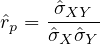 | (58) |
where
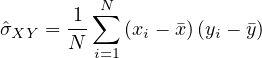 | (59) |
with
 p = 0.93 between the two series! When it is 1, this is a perfect correlation, 0 no correlation, and -1
an anti-correlation. The factor Fcovid is therefore very strongly correlated with the number of deaths
from COVID-19 per 100,000 inhabitants, whatever the country, region, city, or even a boat !!! Under
these conditions, it can be expected that:
p = 0.93 between the two series! When it is 1, this is a perfect correlation, 0 no correlation, and -1
an anti-correlation. The factor Fcovid is therefore very strongly correlated with the number of deaths
from COVID-19 per 100,000 inhabitants, whatever the country, region, city, or even a boat !!! Under
these conditions, it can be expected that:
In conclusion, the epidemic is not going to have a significant impact in most countries of the world, and especially in Africa as the WHO has expressed concern. It is a problem of big cities with old populations. Moreover, gatherings, such as cruises are to be avoided as long as there is no vaccine. Airplane flights are also a problem, due to the temporary high concentration of the population. Until a vaccine is found, all countries currently concerned will remain very fragile.
There are many quantities to quantify the risk associated to an outbreak: the risk of being contaminated, the risk of being very sick, the risk to be in intensive care units and the risk of death. It can be defined per any object, the object being a people, a boat, a meeting, a city, an area or a country.
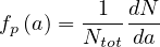
If dN∕da is the elementary number of people per age group in a country of Ntot people,
 | (64) |
or
 | (65) |
where
 | (66) |
is the normalized age structure.
For a given age group, the risk of deaths is
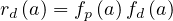 | (67) |
where fd is the absolute fraction of contaminated people who will die from the COVID-19, since
fatality is strongly age-dependent. Here, fd
is the absolute fraction of contaminated people who will die from the COVID-19, since
fatality is strongly age-dependent. Here, fd is given by the relative distribution of deaths [6],
normalized to the mean value of the estimated fatality rate δd, i.e.
is given by the relative distribution of deaths [6],
normalized to the mean value of the estimated fatality rate δd, i.e.
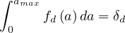 | (68) |
Regarding the studies performed recently, δd = 0.7% deduced from the Diamond-Princess cruise liner case is a robuste reference.
Therefore for a whole country, knowing the age structure, the total risk of deaths is the integral over the ages,
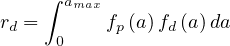 | (69) |
and this parameter alows to compare the risk of oubreak between different countries or world areas, which have different age structures. It is therefore straightforward to estimate that the risk is small in Africa, since most of the population is young, and much more critical in Europe.
It is well known that population density is a major factor in the development of an outbreak, since in high density areas, the risk of interaction between people, and so for contamination. This is the reason why cities with high population densities are the main foci of the outbreak.
With similarities with cross-section theory, the probability of interaction for a test person is the product of the local population density n times the effective surface σ of this person (cross-section). This number may be also a function of the age, if some societal distanciation may take place naturally (old persons are living close or far from the rest of the family)
 | (70) |
Therefore,
 | (71) |
and integrating over the age, the local risk of deaths is
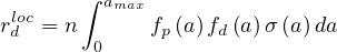 | (72) |
For a city like Paris, with n = 20000∕km2 = 0.02∕m2, the mean surface per people is S = 1∕n = 50m22. Even if the density is high, the mean surface is much larger than the surface of interaction corresponding to the vertical projection of the body of a person, which can be estimated to s = 0.78m2. Therefore, only binary interaction must be considered.
Ultimately, the number of deaths for a given city is
 | (73) |
or for Paris, with Nloc ≃ 2.2 × 10+6 inhabitants, and neglecting age structure Ndloc = Nlocδdsn ≃ 240. It
is below the absolute osbervation which is about 1450 the 27th of April 2020, which allows to estimate
the effective surface of interaction in the ratio 1450∕240 = 6. Considering that the surface of
interaction in the lockdown is σlockdown = 4.5m2, the number of deaths at Lyon and Marseille should
be only 140 and 87 respectively, which is close to observations at the save date, since their density and
populations are  and
and 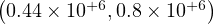 . At Wuhan, with is population
of Nloc ≃ 11 × 10+6 and a density of n = 0.00582∕m2, the total estimated number of deaths is 2000
very close to the observed value around 2570.
. At Wuhan, with is population
of Nloc ≃ 11 × 10+6 and a density of n = 0.00582∕m2, the total estimated number of deaths is 2000
very close to the observed value around 2570.
Without lockdown, the surface of interaction is much larger. If the total number of people that can be contaminated is about 60% of the population before the natural end of the outbreak thanks to a value of R0 ≃ 3 for the COVID-19, the number of deaths should be 9240. So surface of interaction is σfree = 9240 × σlockdown∕1450 = 28m2, about half the mean surface in Paris. The estimated R0 = τiσfree∕S = 3.6 and in the lowkdown phase R0 = τiσlockdown∕S = 0.57 close to the observations. The fact that the estimated R0 values match those of France suggested that the effective surface of interaction of people is almost universal, in the lockdown or free phases.
Concerning a differential distanciation, it can be modeled according to the law
 | (74) |
for a < aref,and where σlockdown < σ < σfree depending upon the strength of the lockdown, and
σ = σlockdown for a > aref. There are some arbitrariness in the determination of aref, but it could
be place after 75 years old.
= σlockdown for a > aref. There are some arbitrariness in the determination of aref, but it could
be place after 75 years old.
In March 2014, a major outbreak of the virus Ebola started in Guinea and spread rapidly in neighboring countries like Liberia and Sierra Leone. It is a viral haemorrhagic fever of humans, with a very high fatality rate, around δd = 50%, about hundred time what is estimated for the virus SARS-cov-2. The dynamics of the outbreak is different from COVID-19, since mean incubation time is about τi = 10 days (ranging between 2 and 20 days), while itis τi = 4 days approximately. The main difference is that durong the incubation period, sick people may contaminate other people for the SARS-cov-2 virus, while in principle, the contamination is only possible if first symptoms appear. Furthermore, a very close physical contact is necessary for a contamination by the Ebola virus, while, oral transmission is likely the main process for the SARS-cov-2.
The example of Liberia is considered, since the number of cases is rather large, making statistics quite accurate. This example allows to investigate the capability of the model to describe this type of outbreak, and if from data, standard R0 can be retrieved. In addition, it is important to test the case where likely the number of tested cases if well known, since all sick people are rapidly well diagnosed, and the chain of contamination may be rather well known.
As shown in Fig. 102, the whole outbreak can be well reproduced by the model, despite its simplicity. As for the SARS-cov-2, it is a multi-steps outbreak, as observed in many countries, with a major propagation after day 71, while initial evolution suggested that the Ebola outbreak was totally controlled. From the early phase of the second rise and taking an averaged time of contamination of 3 days (before death in general), R0 ≃ 1.5 approximately, close to the values that have been estimated. Therefore the contagiosity of Ebola virus is much less than SARS-cov-2. This is likely because the transmission of Ebola virus requires physical contacts with the sick person and possibly its infected fluids, while for SARS-cov-2, it is likely mainly aerial transmission in addition to physical one on surfaces. Consequently, only 33% must be immunited by a vaccine, to protect the whole population from Ebola virus. Furthermore, R0 is rather low since people that have symptoms die rapidly. So this cut quickly the probability of transmission. In that sense, even if the rate of mortality of Ebola virus is extremely high, it is less dangerous at the world scale than VIH or SARS-cov-2 viruses.
From Fig. 102, it can be shown that the cumulative number of certified cases is consistent with the deaths number, over the whole outbreak duration. The good agreement is the consequence of the process of contamination, which allows to track more easily sick people, because physical contact is necessary.
A long tail of low level daily cases and deaths is observed during several months, with some similarities with South-Korea, as shown in Fig. 103. This highlights the need of a strong control of the outbreak during many months for the COVID-19, and the need not to relax the efforts made. The occurence of the peak in the outbreak is just a step in the global management of the virus spread. Permanent control will be likely necessary, regarding the high reproduction factor R0 of the SARS-cov-2, as compared to Ebola virus.
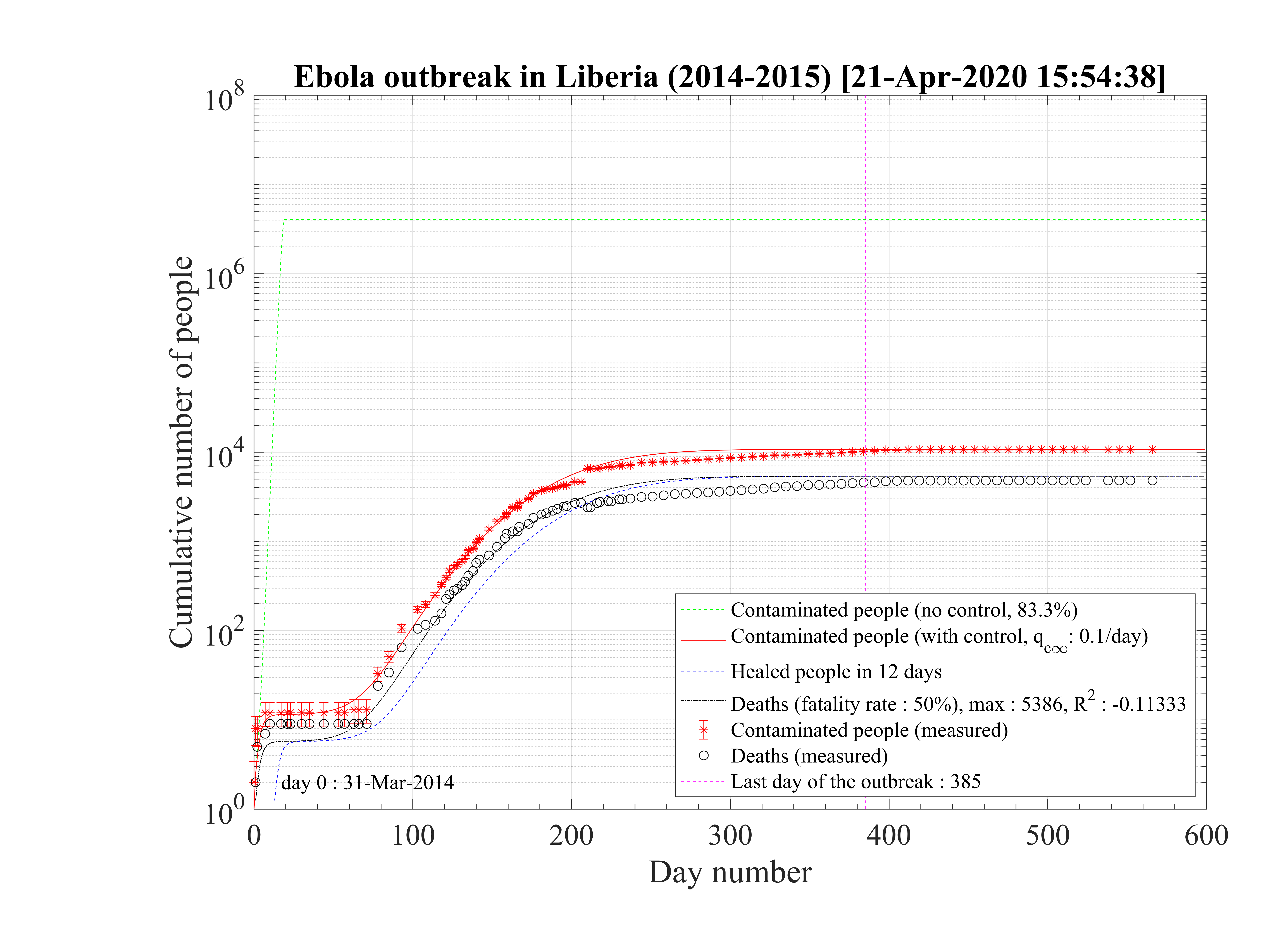
A simple zero-dimension model of the coronavirus outbreak has been developped, and is able to give indications on the near future if the daily trend of the cumulative number of contaminated people is confirmed. As this model is general, it has been successfuly tested against the seasonal flue, and with standard simulation parameters, the 10000 deaths per year in France is well recovered.
At the date of the 6th of March, there is no control of the outbreak in France, and all citizen will face the disease if nothing is changing in the management of the outbreak. The number of deaths will be extremely large, and the health care units totaly overloaded during several months. Such a situation is similar in Italy, and in this country the situation is worse, since the mortality rate seems to be much higher, about 4%, like in China, while it is about 1.5% only in France. The situation is simular in Switzerland but with a much lower fatality rate. In South-Korea, though the outbreak is not totally stabilized, the evolution is favorable thanks to the quarantine, and it should stop after 120 days from the model. In Iran, the outbreak is not yet stabilized, but the authorities have clearly acted, but very late as compared to other countries, leading to a very large number of ill people, and deaths. The outbreak in Spain and USA are very similar in their respective time evolutions.
In China, where the model have been successfully applied too, the residual rate of contamination has been drastically lowered to qc∞ = 0.001 by a severe quarantine like in Wuhan city and around in Hubei state, but also elsewhere, each time the virus was emerging suddenly [2]. This approach was successful, and from predictions, the outbreak will end in March 2020.
South Korea, faced two phases of the outbreak, and a third one is starting the 18th of March. The second phase of the outbreak whose origin is well identified (large religious meeting), highlights the risk of a restart of the outbreak everywhere it has be stabilized, since most of the population is not immunited against the virus, by the artificial control of the outbreak. Only a massive vaccination campaign may reduce definitively the risk of a periodic restart of the outbreak as it was indicated and observed in South Korea. China is clearly aware of this situation, and the number of certified cases is stable, above expectations, because of external contaminated people entering the country
From the analysis of the eight most concerned countries, some conclusions can be drawn with quantitative numbers. There are two ways to control the disease: (i) without any vaccine available, only a drastic quarantine could reduce the daily contamination rate. This option seems not considered yet (11th of March) by the French governement while Italian one decided it the 8th of March for about one month, regarding the overload of the hospitals. In Italy, the effect of the quarantine are not visible the 11th of March, but a good probability of success like in China will require a strict application of the quarantine. This option is the worse for the economy. (ii) an efficient vaccine is found, and in few weeks, the outbreak is stopped. Unprobable regarding usual time it takes to develop such a medication (about a year).
So, without strong quarantine to reduce drastically the contamination rate qc, a dramatic situation will likely occur in France very soon, and the example of what append in Italy gives clearly indication on what should be done quickly. Nevertheless, the situation between the two countries seems to be different concerning the number of deaths, since it is significantly higher in Italy than in France.
The fatality rate is subject to different values from countries to countries, with similar health care systems. This may result from the level of activity of old people within the society. The virus is spreading actively, concerning all classes of age, but older people are much more sensitive to severe form of the disease. The elderly must be isolated from young children to reduce the risk of contamination.
Based on the modeling of the outbreak in the line cruiser Diamond Princess, a low fatality rate is estimated, about 1.0%, close to South-Korea. In this case, the number of contaminated people is know exactly. The surprizing low fatality rate despite of the old mean age of the passengers, may indicate that the co-morbidity is the key aspect of the age dependence of the fatality rate that has been estimated in China. If the number of deaths is the reference to estimate the outbreak time evolution, the number of contaminated people is strongly under-estimated, as this number is growing. Nevertheless, the time evolution of the number of people requiring respiratory support in continuous health care units is not well reproduced. At the time of the 13th of March, it is not possible to decide if this low fatality rate scenario is effectively realistic.
If the coronavirus is seasonal like the flue, this would be an extraordinary chance. In that case, the outbreak will stop naturally quite quickly. Nothing tends to prove this fact at present time, since it develops in countries with have hot and cold weather too. The evolution of the virus in Africa will be very interesting from this point of view.
It is important to notice from WHO data, that the outbreak has almost always a quiescent phase of several days (or weeks) because the virus is first imported by travellers using fast and long distance transportation systems that are efficiently detected at the airport principaly (Levy flight effect). Once the outbreak becomes domestic, the local growth of the number of contaminated people becomes rapidly dramatically high.
Most of the people believe that the coronavirus is a marginal problem, as compared to the annual flu, or even the Spanish flu in 1918. When calculations are performed from the model with values successfully compared to observations, it is possible to see that the coronavirus is a very serious health problem at the world scale. It should be recalled that the Spanish flu in 1918 killed Nd = 218000 persons in France. At that time, Ntot = 38.67 × 10⁶, so the ratio Ndflu∕Ntot = 0.56% (to the whole population), while for the coronavirus, it may reached Ndcoronavirus∕Ntot = 1 - 1.5%, so twice or three times more if the outbreak is uncontrolled. The new coronavirus outbreak is therefore a major event, and not a small problem, and could be worse than the Spanish flu, which killed between 50 and 60 millions of people over the world. This is particularly critiacal if mortility rates in China and Italy are considered and widespread. The initial reproducton factor R0 of the coronavirus outbreak is estimated to 5 apprimately, twice more than the Spanish flue [7].
Finally, there is an important difference between the Spanish flue and the coronavirus outbreak until no vaccine have been found for the later. Indeed, for the Spanish flu, the disease has disappeared naturally, because the aggressivity of the virus has progressively decreased during the outbreak, a well known behaviour, and because the probability of contamination pc has also decreased substantially since many people have been contaminated (immunity) or died. For the coronavirus, pc is still close to unity at the time the report is written, which mean that the reservoir of people that can be still contaminated is very high. So the outbreak may restart very quickly is no active and permanent watch is not achieved everywhere in the world. An example is the Ebola virus, which periodically appears in Africa, and remain very contagious. Therefore, the success in controlling the coronavirus outbreak in China does not mean that the whole effort is achieved, and the standard life can restart as usual. Considerable care should be taken in all the countries. The two phases of the outbreak in South-Korea are a good example of the fragility of the situation, once the outbreak is ended by quarantine.
Ultimately, the case where the coronavirus outbreak would have been like the seasonal flu, with a fatality rate of 0.1%, has been considered. In this case the number of officialy contaminated people is totally underestimated, it is possible to reproduce it for France, day zero being the 10th of February. The contamination rate should be very high and constant qc0 = qc∞ = 0.4, and the number of people requiring an active ventilation in continuous health care units must exceeds the number of available respirators by mid of March. The hypothetic number of contaminated people is about 65000 at the date of the 11th of March. All the population should be immunited by end of March, and 47000 people should die from the outbreak, that’s much higher than the seasonal flu, because of the much higher contamination rate to reproduce the daily increase of deaths. Coming two weeks should be crucial to conclude about the two scenarii at the date of the 13th of March.
The study of the Ebola outbreak in West Africa during 2014-2015 shows the ability of the model. It gives a rather good estimate of the reporduction factor R0 = 1.5, and with a constant fatality rate, the cumulative number of certified cases and deaths may be well reproduced. A tail of daily cases and deaths before the full end of the outbreak is observed, which clearly indicates the need to maintain strict survey during many months after the peak to avoid a possible restart of the outbreak.
A very interesting and well documented french article on the Covid-19 outbreak. One of the best document on the COVID-19 ever seen can be obtained here. Another intersting link of a standard SIR modeling, which gives indication how to fight COVID-19.
I would like to thanks Pr. Luca Mercalli, President and Editor in Chief Societ`a Meteorologica Italiana onlus / Nimbus journal, for his continuous support and his help to get some data from Italy.
[1] Wang et al., Cell Discovery (2020)6:11
[2] Lai et al., medRxiv 2020.03.03.20029843; doi: https://doi.org/10.1101/2020.03.03.20029843
[3] Biggerstaff et al., BMC Infectious Diseases 2014, 14:480
[4] Liu et al., Journal of Travel Medicine, 2020, 1–4
[5] Zhao S et al., Int J Infect Dis. 2020 Mar;92:214-217. doi: 10.1016/j.ijid.2020.01.050. Epub 2020 Jan 30.
[6] Wu Z, McGoogan JM., JAMA. 2020 Feb 24. doi: 10.1001/jama.2020.2648. [Epub ahead of print]
[7] Du Z et al. Emerg Infect Dis. 2020 Jun
[8] Qun L. et al., N Engl J Med 2020;382:1199-207. DOI: 10.1056/NEJMoa2001316